library(tidyverse)Problem Set 6: The Law of Large Numbers and the Central Limit Theorem
Not graded. This is only for you to reinforce content from Weeks 4 to 6, since there is no graded problem set the week of an exam. Answers are in the drop-downs; try each part before you open them.
TipReview Quant Camp as you go
This set leans on the R you learned at Quant Camp. When you get stuck on filtering, grouping, or plotting, go back to the Quant Camp materials. They’re the fastest way to get unstuck.
Libraries you will need:
Question 1: Election night, counted one ballot at a time
On election night, each county counts its ballots one by one, and the TV networks report the running share for candidate A. Suppose every ballot is a vote for A with probability 0.52, independently of the others. (So A really is ahead.)
- Simulate election night in 20 counties, each counting 5,000 ballots. For each county, compute A’s running share after every ballot (the share of the ballots counted so far that went to A). Plot the 20 running shares, as in lecture’s funnel of 20 people rolling dice, with a horizontal line at 0.52 and the x-axis on a log scale. (Hint:
rbinom(n, size = 1, prob = 0.52)makesnballots, andcumsum()adds them up as you go.)
TipAnswer
set.seed(211)
counts = expand_grid(county = 1:20, ballot = 1:5000) |>
  mutate(vote_a = rbinom(n(), size = 1, prob = 0.52)) |>
  group_by(county) |>
  mutate(share_a = cumsum(vote_a) / ballot) |>
  ungroup()

ggplot(counts, aes(x = ballot, y = share_a, group = county)) +
  geom_hline(yintercept = 0.52, color = "orange", linewidth = 1.2) +
  geom_line(alpha = 0.5) +
  scale_x_log10() +
  labs(x = "Ballots counted so far (log scale)", y = "A's share so far")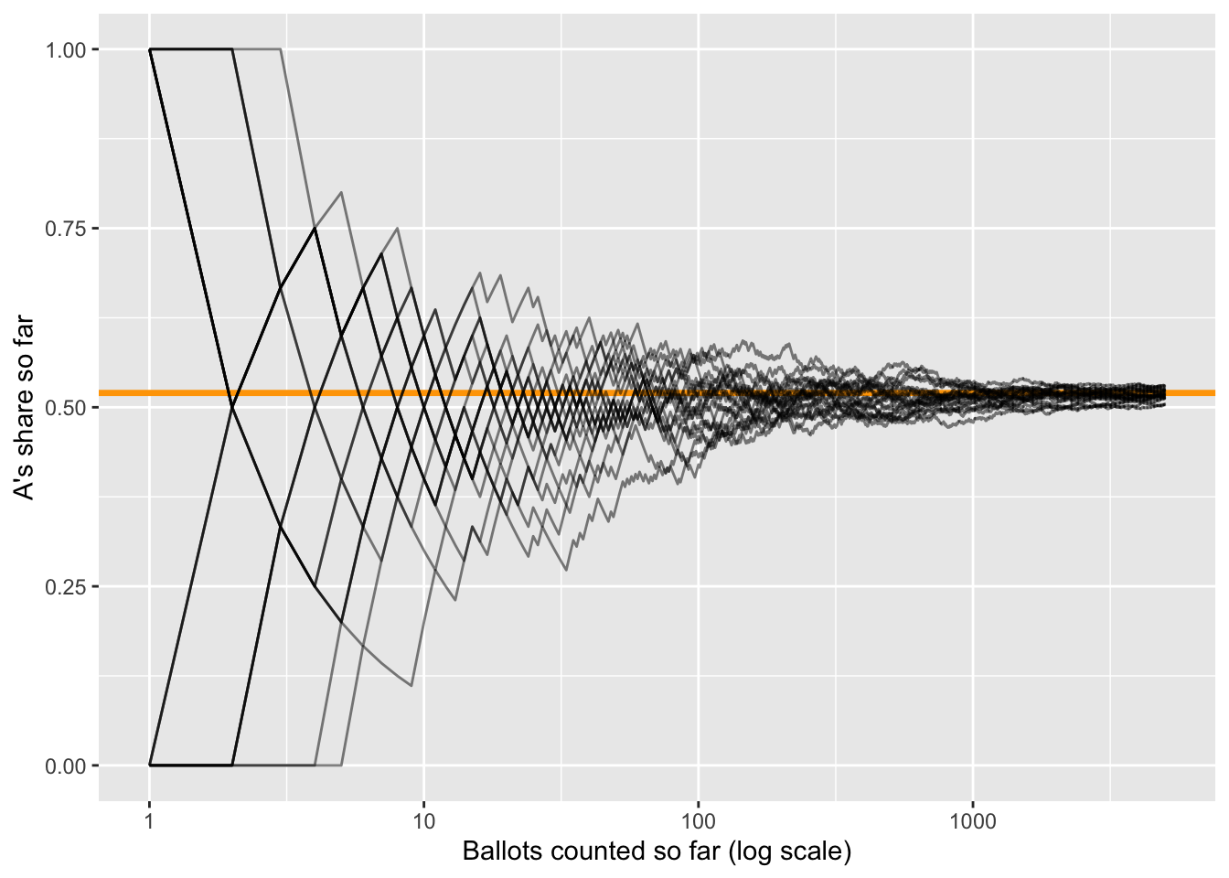
Every county’s running share closes in on 0.52: the law of large numbers, for a 0/1 outcome. Early on, the shares are all over the place (after one ballot, A has either 0% or 100%).
- Add the band that week 5’s formula predicts: \(0.52 \pm 2 \sqrt{p(1 - p)/n}\), with \(p = 0.52\) and \(n\) the number of ballots counted so far. Do the running shares stay inside it?
TipAnswer
band = tibble(ballot = 1:5000) |>
  mutate(se = sqrt(0.52 * 0.48 / ballot),
         upper = 0.52 + 2 * se,
         lower = 0.52 - 2 * se)

ggplot(counts, aes(x = ballot)) +
  geom_line(aes(y = share_a, group = county), alpha = 0.3) +
  geom_hline(yintercept = 0.52, color = "orange", linewidth = 1) +
  geom_line(data = band, aes(y = upper), color = "goldenrod", linewidth = 1.2, linetype = "dashed") +
  geom_line(data = band, aes(y = lower), color = "goldenrod", linewidth = 1.2, linetype = "dashed") +
  scale_x_log10() +
  coord_cartesian(ylim = c(0, 1)) +
  labs(x = "Ballots counted so far (log scale)", y = "A's share so far")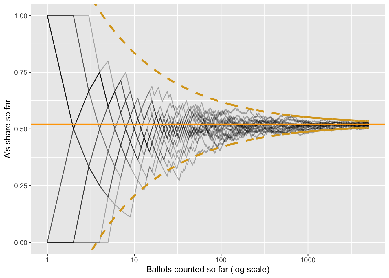
Almost all of them. The band is the funnel from lecture, for a coin flip with \(p = 0.52\): its width shrinks like \(1/\sqrt{n}\).
- How many ballots does a county have to count before the band is within 2 percentage points of 0.52 on each side? Solve \(2\sqrt{0.52 \times 0.48 / n} = 0.02\) for \(n\).
TipAnswer
\[ 2\sqrt{\frac{0.2496}{n}} = 0.02 \quad \Rightarrow \quad \frac{0.2496}{n} = 0.0001 \quad \Rightarrow \quad n = 2{,}496 \]
About 2,500 ballots. To halve the band to 1 point, you’d need four times as many: about 10,000.
- Early in the count, some counties show A losing, even though A is ahead in every county. Use the plot to explain why networks wait before calling a close race, and why waiting works.
TipAnswer
With a few hundred ballots counted, the running share can easily be several points from 0.52, so a county can show A below 50% by chance. That’s the left side of the funnel. Waiting works because of the LLN: as the count grows, the running share settles on A’s true share, and the band narrows until it no longer includes 50%.
Question 2: Chebyshev’s inequality, with numbers
Household incomes in a county have a mean of $60,000 and an SD of $20,000. We know nothing else about their distribution: they could be skewed, lumpy, anything.
NoteWhat the symbols mean
Chebyshev’s inequality comes in two versions in this question:
\[ \underbrace{P(|X - \mu| \geq k\sigma) \leq \frac{1}{k^2}}_{\text{one household}} \qquad\qquad \underbrace{P(|\bar{X} - \mu| \geq \varepsilon) \leq \frac{\sigma^2}{n \, \varepsilon^2}}_{\text{the average of } n \text{ households}} \]
| Symbol | What it is | In this question |
|---|---|---|
| \(X\) | One household’s income: a random variable | |
| \(\mu\) | The mean of \(X\) | $60,000 |
| \(\sigma\) | The SD of \(X\) (\(\sigma^2\) is its variance) | $20,000 |
| \(\lvert X - \mu \rvert\) | How far a household is from the mean, in either direction | |
| \(k\) | How many SDs from the mean counts as “far” | 2 or 3, in part (a) |
| \(P(\ldots)\) | The chance of what’s inside: here, the share of households that far out | |
| \(\bar{X}\) | The average income of \(n\) households in a survey | |
| \(n\) | The number of households surveyed | 400, 1,600, or 10,000, in part (c) |
| \(\varepsilon\) | How far off counts as a “big miss,” in dollars | $2,000, in part (c) |
Both say the same thing: a small spread leaves room for only a few values far from the mean.
- Use Chebyshev’s inequality, \(P(|X - \mu| \geq k\sigma) \leq 1/k^2\), to find the most households that can earn $20,000 or less or $100,000 or more. Then the most that can earn $0 or less or $120,000 or more. (Hint: how many SDs from the mean is each cutoff?)
TipAnswer
$20,000 and $100,000 are each $40,000 from the mean: 2 SDs. So at most \(1/2^2 = 1/4\), or 25%, of households can be that far out.
$0 and $120,000 are each $60,000 from the mean: 3 SDs. So at most \(1/3^2 = 1/9\), about 11%.
- If incomes were normal, what share would actually be 2 or more SDs from the mean? 3 or more? Use
pnorm(). Why are Chebyshev’s caps so much bigger?
TipAnswer
# 2 or more SDs out: $20,000 or less, plus $100,000 or more
pnorm(20000, mean = 60000, sd = 20000) + (1 - pnorm(100000, mean = 60000, sd = 20000))
[1] 0.04550026# 3 or more SDs out: $0 or less, plus $120,000 or more
pnorm(0, mean = 60000, sd = 20000) + (1 - pnorm(120000, mean = 60000, sd = 20000))[1] 0.002699796About 4.6% and 0.3%, against Chebyshev’s 25% and 11%. Chebyshev’s cap has to hold for every distribution, however lopsided, so it can’t use anything about the normal’s thin tails. Its only input is the variance. That’s the price of assuming nothing about the shape.
Now a survey samples \(n\) households and reports their average income, \(\bar{X}\). Use the version of Chebyshev for an average,
\[ P(|\bar{X} - \mu| \geq \varepsilon) \leq \frac{\sigma^2}{n \, \varepsilon^2}, \]
to find the most a survey can miss the county’s mean by $2,000 or more, for \(n\) = 400, 1,600, and 10,000 households. Write out the numbers plugged in.
TipAnswer
\(\sigma^2 = 20{,}000^2 = 400{,}000{,}000\) and \(\varepsilon^2 = 2{,}000^2 = 4{,}000{,}000\), so \(\sigma^2 / \varepsilon^2 = 100\) and the cap is \(100 / n\):
\[ n = 400: \;\; \frac{100}{400} = 0.25 \qquad n = 1{,}600: \;\; \frac{100}{1{,}600} \approx 0.06 \qquad n = 10{,}000: \;\; \frac{100}{10{,}000} = 0.01 \]
At most 25%, 6%, and 1% of surveys miss by $2,000 or more. The cap shrinks like \(1/n\): that’s the law of large numbers.
- How many households does the survey need so that at most 5% of surveys miss by $2,000 or more?
TipAnswer
Set the cap equal to 0.05 and solve: \(100 / n = 0.05\), so \(n = 2{,}000\) households. Any \(n\) of 2,000 or more guarantees it, whatever the shape of the income distribution.
Question 3: A poll’s sampling distribution, and what the normal tells us
A ballot measure has the support of 52% of a city’s voters. A pollster surveys 600 randomly chosen voters and reports \(\hat{p}\), the share who support it.
- Simulate 10,000 polls of 600 voters each and plot the sampling distribution of \(\hat{p}\). What are its center and its SD? Compare the SD to week 5’s formula, \(\sqrt{p(1 - p) / n}\).
TipAnswer
set.seed(211)
polls = tibble(poll = 1:10000) |>
  mutate(p_hat = map_dbl(poll, \(i) mean(rbinom(600, size = 1, prob = 0.52))))

ggplot(polls, aes(x = p_hat)) +
  geom_histogram(binwidth = 0.005, color = "white") +
  geom_vline(xintercept = 0.52, color = "orange", linewidth = 1.2) +
  labs(x = "Share supporting the measure in one poll", y = "Polls (out of 10,000)")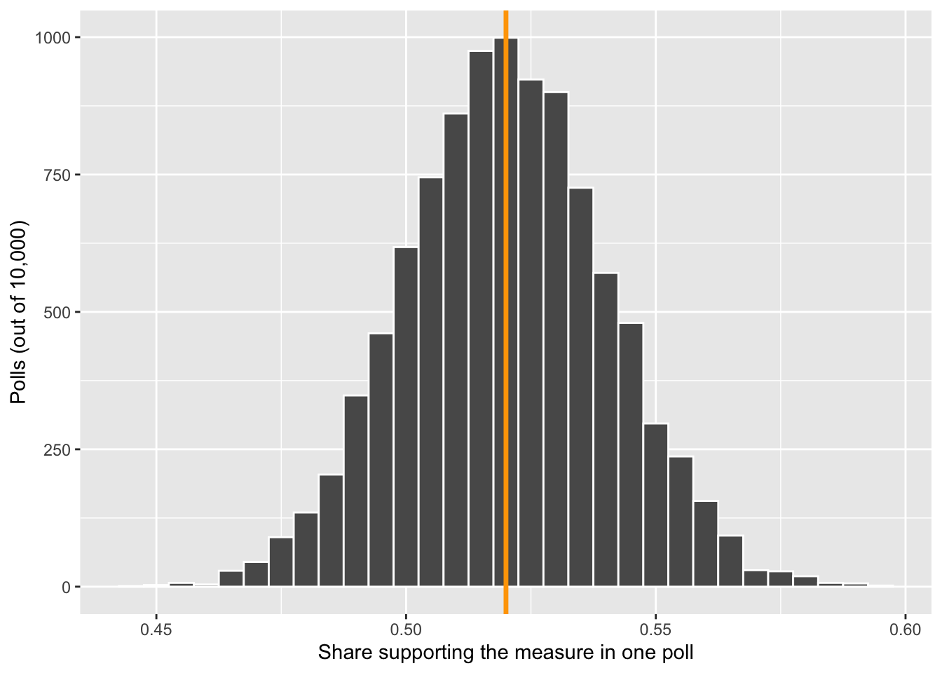
polls |>
  summarize(center = mean(p_hat), sd = sd(p_hat))
# A tibble: 1 × 2
center sd
<dbl> <dbl>
1 0.520 0.0203se_poll = sqrt(0.52 * 0.48 / 600)
se_poll[1] 0.02039608The center is 0.52 (the estimator is unbiased) and the SD is about 0.020, which matches the formula: a typical poll lands about 2 points from the truth. The shape is a bell, by the CLT.
- Between what two values do the middle 95% of polls fall? Use
qnorm(), then check it againstquantile()on your simulated polls.
TipAnswer
qnorm(c(0.025, 0.975), mean = 0.52, sd = se_poll) # the normal[1] 0.4800244 0.5599756quantile(polls$p_hat, c(0.025, 0.975)) # simulation 2.5% 97.5%
0.48 0.56 From about 0.48 to 0.56: \(0.52 \pm 1.96 \times 0.020\). The two methods agree.
Question 4: Arrests, and a bell from a lopsided start
rpois() draws from a Poisson distribution, a common model for counts of events: 0, 1, 2, 3, and so on, with no upper limit. It has one parameter, lambda, and both its mean and its variance equal lambda.
Suppose the number of arrests in a small town in one week is Poisson with lambda = 2.
- Draw 1,000 weeks with
rpois(1000, lambda = 2). Make a bar chart of the counts. Check that the mean and the variance are both close to 2. Is the distribution symmetric?
TipAnswer
set.seed(211)
weeks = tibble(arrests = rpois(1000, lambda = 2))

ggplot(weeks, aes(x = arrests)) +
  geom_bar() +
  labs(x = "Arrests in one week", y = "Weeks (out of 1,000)")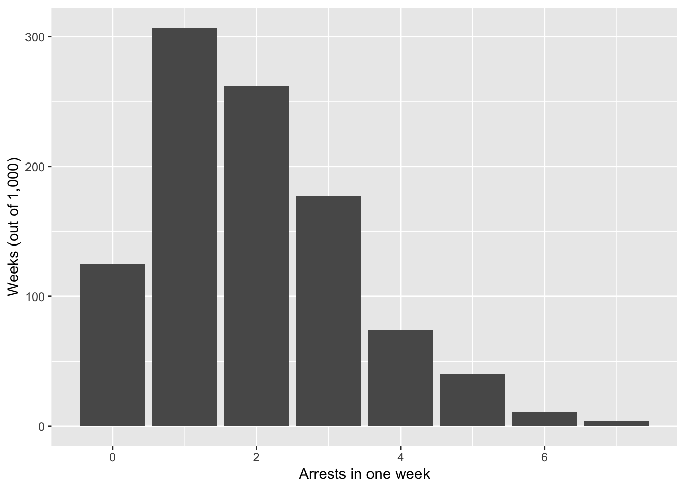
weeks |>
  summarize(mean = mean(arrests), var = var(arrests))
# A tibble: 1 × 2
mean var
<dbl> <dbl>
1 1.95 1.92Both are about 2. The distribution isn’t symmetric: it can’t go below 0 but has a long tail to the right (some weeks have 6 or 7 arrests).
- Now take the average number of arrests over \(n\) weeks. For \(n\) = 1, 5, 30, and 200, compute the average 1,000 times and plot the four distributions side by side. At what \(n\) does the average look like a bell?
TipAnswer
set.seed(211)
averages = expand_grid(n = c(1, 5, 30, 200), run = 1:1000) |>
  mutate(average = map_dbl(n, \(k) mean(rpois(k, lambda = 2))))

ggplot(averages, aes(x = average)) +
  geom_histogram(bins = 30, color = "white") +
  facet_wrap(~n, scales = "free", labeller = label_both) +
  labs(x = "Average arrests per week", y = "Reruns (out of 1,000)")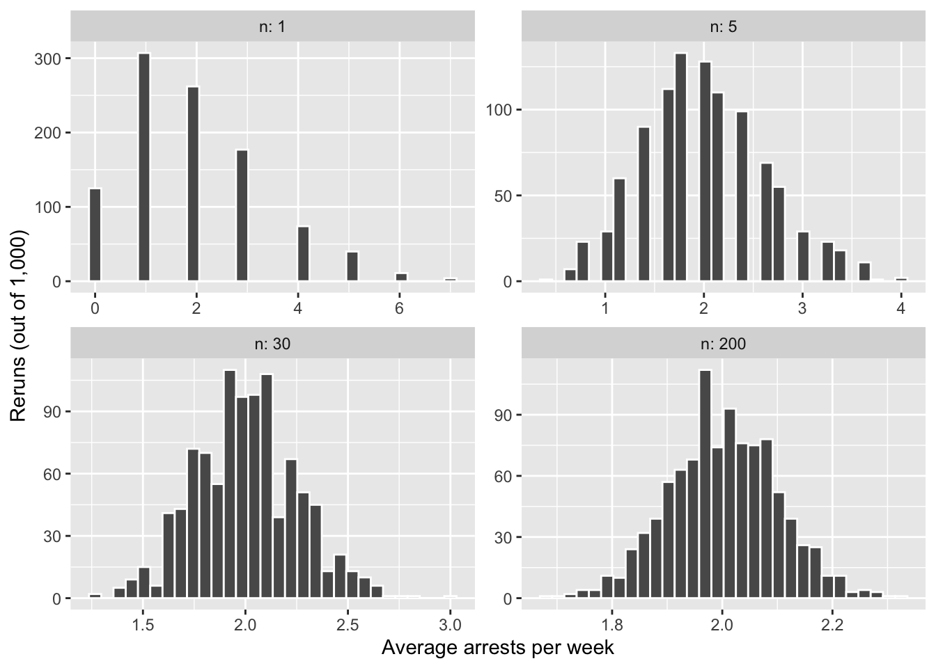
At \(n = 1\) it’s the lopsided Poisson itself. By \(n = 5\) it’s already roughly symmetric, and by \(n = 30\) it’s a bell. That’s the central limit theorem: the average of many independent draws is about normal, whatever one draw looks like.
- Compare the SD of your 200-week averages to what week 5’s formula says it should be, \(\sigma / \sqrt{n}\). (Remember: for a Poisson, the variance is
lambda.)
TipAnswer
averages |>
  filter(n == 200) |>
  summarize(sd = sd(average))
# A tibble: 1 × 1
sd
<dbl>
1 0.0986sqrt(2) / sqrt(200) # sigma = sqrt(lambda)[1] 0.1Both are about 0.10. The formula needs no normality: only the variance of one draw, here \(\sigma^2 = \lambda = 2\).
Question 5: How small can a study get?
A study finds that a civic-education program raises scores on a political-knowledge test by 4 points. Suppose that’s the true effect. Test scores have an SD of 15 points in both the program group and the control group, and the study has 300 people in each group.
- Use week 5’s formula for the standard error of a difference in means, \(\sqrt{\sigma^2 / n_1 + \sigma^2 / n_0}\), to find the study’s standard error.
TipAnswer
\[ SE = \sqrt{\frac{15^2}{300} + \frac{15^2}{300}} = \sqrt{0.75 + 0.75} = \sqrt{1.5} \approx 1.22 \]
- The sampling distribution is about normal (the CLT). Between what two values will 95% of studies like this one land?
TipAnswer
se_study = sqrt(15^2 / 300 + 15^2 / 300)
4 + c(-1.96, 1.96) * se_study
[1] 1.5995 6.4005From about 1.6 to 6.4 points: \(4 \pm 1.96 \times 1.22\). Every study in that range finds a positive effect.
- Now shrink the study. With how many people per group (or fewer) does that 95% range include zero? (Hint: find the group size where \(4 - 1.96 \times SE = 0\). Solving by trial and error in R is fine.)
TipAnswer
# the lower end of the 95% range, for group sizes from 50 to 300
tibble(per_group = 50:300) |>
  mutate(se = sqrt(15^2 / per_group + 15^2 / per_group),
         lower = 4 - 1.96 * se) |>
  filter(lower <= 0) |>
  slice_max(per_group)
# A tibble: 1 × 3
per_group se lower
<int> <dbl> <dbl>
1 108 2.04 -0.000833With 108 people per group or fewer, the lower end of the range reaches zero. By hand: \(1.96 \sqrt{450 / m} = 4\) gives \(m = 450 \times (1.96 / 4)^2 \approx 108\).
- In substantive terms, what do we lose in that world? The program works just as well (the true effect is still 4). What can no longer be said about studies of that size?
TipAnswer
We lose the ability to say that 95% of studies will find a positive effect. With 108 or fewer people per group, more than 2.5% of studies will land at zero or below, finding no effect or a negative one, purely by chance, even though the program really works. A researcher who runs one such study can’t rule out that the effect is zero: the effect is real, but the study is too small to show it reliably. Remember: small studies don’t make effects smaller; they make them harder to distinguish from zero (or opposite effects).