library(tidyverse)Problem Set 4: Random Variables and the Sampling Distribution
Due: Monday, October 26 by 11:59 PM. Email both your .qmd and your rendered .html to Max Welch (mwelch@ucdavis.edu).
TipReview Quant Camp as you go
This set leans on the R you learned at Quant Camp. When you get stuck on filtering, grouping, or plotting, go back to the Quant Camp materials. They’re the fastest way to get unstuck.
ImportantUsing AI
Use AI the way people used Google, R’s help pages, and Stack Overflow before AI: ask precise, limited questions to get unstuck on part of a question. Passing off AI-generated work wholesale as your own is not allowed. See the syllabus and the Department’s policy on generative AI.
Format: Write your answers in one Quarto document, saved in the sets/ folder of your course project. Start it with this header, so the HTML renders as one self-contained file:
---
title: "Problem Set 4"
author: "Your name"
format:
  html:
    embed-resources: true
---
Your document should read as a short report: brief prose explaining your reasoning, not just code and output.
This set is shorter than the others, since the exam took half of class.
Libraries you will need:
WarningMethods subfield
Parts marked Methods portfolio are required if you plan to choose methods as a subfield. They’re optional, and recommended, for everyone else.
Question 1: An election as a random variable
A country is holding an election between four parties: A, B, C, and D. The polls say B and C are tied for first, with 35% of the vote each, and A and D are tied for last, with 15% each.
One voter walks into the booth and picks a party. In the language of lecture, what is the experiment and what is the sample space?
Define a random variable, \(Y\), for whether the voter picks party B or not. What is the probability distribution of \(Y\)? And how is it distributed (e.g., what family)?
Define a second random variable, \(W\), for whether the voter picks a front-runner party. What is the probability distribution of \(W\)? And how is it distributed (e.g., what family)?
Now, say we have 1,000 voters. Define a random variable, \(V\), for whether B wins the election. How is \(V\) distributed (what family)? What do you think its probability distribution is, and why? (Hint: you can’t compute it exactly, but think about how B and C compare.)
Simulate one election of 1,000 voters.
sample()can give each item its own chance (see below), the wayrbinom()gave each unit its own chance in Problem Set 2. You want to make a tibble of 1,000 voters, and then for each row, mutate which party the person voted for.set.seed(211) sample(x = c("Joe", "Sam", "Brian"), size = 10, replace = TRUE, prob = c(.9, .05, .05))Notesample()withprobEach draw picks one item from the list, with the chances in
prob(in the same order as the items).replace = TRUEputs the item back after each draw, so one voter’s choice doesn’t change the next voter’s chances. Withoutprob, every item has the same chance; that’s how we usedsample()in lecture.Compute each party’s share of the vote. Who won? Do the shares match the polls (15/35/35/15) exactly? Why or why not?
Question 2: Three plots, three different things
A research team runs a survey of 5,000 households, asking each one its yearly income. We made the data up, so we can rerun the survey as often as we like. The three figures below come from that survey.
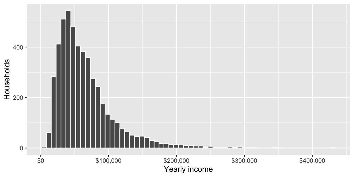
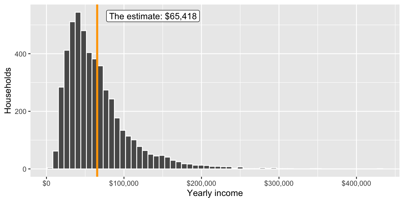
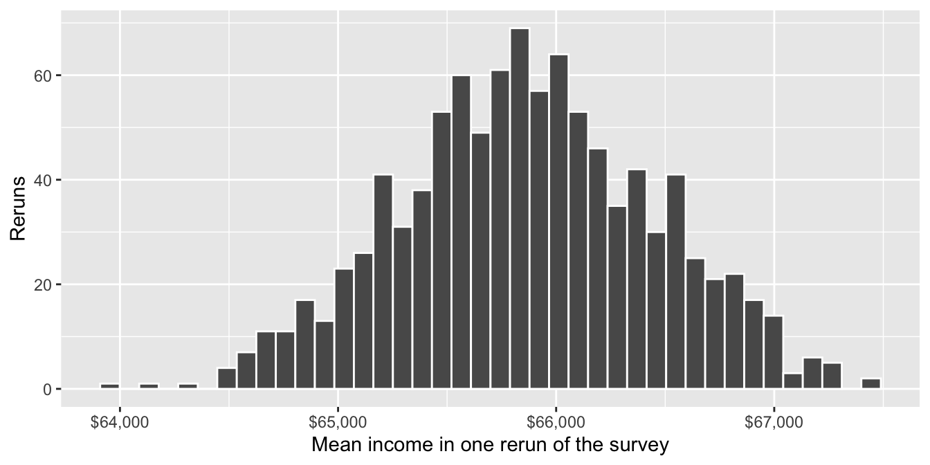
Explain how the three plots differ: what is each plotting? Which of the three figures could a researcher who ran this survey once see with real data? Which figure does a standard error describe?
Figure 1 is wide and skewed to the right. Figure 3 is narrow and roughly symmetric. Why is Figure 3 so much narrower than Figure 1?
WarningMethods portfolio
- Suppose the survey had 500 households instead of 5,000, and we reran it 1,000 times. Which of the three figures would change, and how? Which would stay about the same? Make a prediction for each, with a reason.
Question 3: Your own DGP, and its sampling distribution
In lecture, we wrote the résumé study as a DGP (make_resumes()), wrapped it in a function that returns one estimate (run_resumes()), and reran it 1,000 times. The code is in the class script, 04-code.R. Here you’ll do the same thing for a study of your own.
Describe your world. Pick a unit (people, counties, countries, bills…), a yes/no treatment, and an outcome that is either 0/1 or a number. Your estimand is the difference in means of the outcome between treated and untreated units: the effect you build into the DGP. Also pick one or two other features of the unit that affect the outcome, the way experience and age affected callbacks. Say what your world is and justify your numbers in a few sentences.
Build the DGP. Copy
make_resumes()from the class script and change it into a function that makes one run of your study, with 1,000 units. Treatment should be assigned by a coin flip, as names were. The systematic part (yourpline, or an equation for a numeric outcome) should include the treatment effect and your other features. The random part is the draw:rbinom()for a 0/1 outcome, orrnorm()for a numeric one. Run the DGP once and compute the difference in means. How far is it from the effect you built in? Why isn’t it exact?Rerun it 1,000 times. Copy
run_resumes()and change it so that one call returns one estimate from your DGP. Rerun it 1,000 times withmap_dbl(), as in lecture, and plot the 1,000 estimates in a histogram with a vertical line at your estimand. What is this plot called?
WarningMethods portfolio
- What drives the variation? In lecture, every rerun made new units and flipped new coins. Now hold the units fixed: make your 1,000 units once, outside the function, and write a new function that only redraws the outcome (the
rbinom()orrnorm()step) for those same units. Rerun it 1,000 times. Compare the standard deviation of these estimates with the standard deviation of the estimates from (c). Are they close? What does that tell you about where most of the randomness in your estimate comes from?