library(tidyverse)
library(juanr)    # afrobarometer
library(socviz) # county_data. If you skipped Quant Camp: install.packages("socviz")Problem Set 3: Averages, Spread, and Relationships
Not graded. This is only for you to reinforce content from Week 3, since there is no graded problem set the week of an exam.
TipReview Quant Camp as you go
This set leans on the R you learned at Quant Camp. When you get stuck on filtering, grouping, or plotting, go back to the Quant Camp materials. They’re the fastest way to get unstuck.
Libraries you will need:
WarningMethods subfield
Parts marked Methods portfolio are required if you plan to choose methods as a subfield. They’re optional, and recommended, for everyone else.
Question 1: Survey weights
afrobarometer (in juanr) is a survey of 2,378 people in Ethiopia, carried out in late 2019 and early 2020. Surveys rarely reach every kind of person in the right proportions, so each respondent has a weight: how many people in the country that respondent stands for, relative to the average respondent. A weight of 2 means the respondent counts twice as much as average; a weight of 0.5, half as much.
- Make a histogram of
weight. What’s the average weight? The smallest and the largest?
TipAnswer
ggplot(afrobarometer, aes(x = weight)) +
  geom_histogram(binwidth = 0.1, boundary = 0, color = "white") +
  labs(x = "Survey weight", y = "Respondents")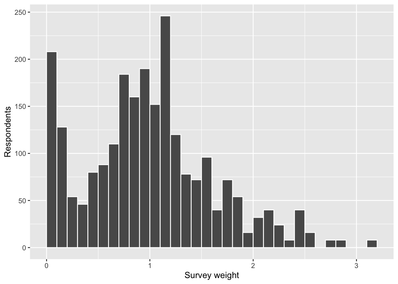
afrobarometer |>
  summarize(mean = mean(weight), min = min(weight), max = max(weight))
# A tibble: 1 × 3
mean min max
<dbl> <dbl> <dbl>
1 1 0.0350 3.14The weights average exactly 1, so a weight reads as “times the average respondent.” Most fall between about 0.5 and 1.5, but some respondents count for almost nothing and the heaviest count about three times as much as average.
- Look at the 20 respondents with the largest weights (
slice_max()is handy here). Usecount()to look at their gender, whether they live in an urban or rural area, their region, and their education. What do they have most in common? Compare with the whole sample.
TipAnswer
top_20 = afrobarometer |>
  slice_max(weight, n = 20)

top_20 |> count(urban)
# A tibble: 1 × 2
urban n
<fct> <int>
1 rural 24afrobarometer |> count(urban) |> mutate(share = n / sum(n))# A tibble: 2 × 3
urban n share
<fct> <int> <dbl>
1 rural 1704 0.717
2 urban 674 0.283top_20 |> count(region)# A tibble: 3 × 2
region n
<fct> <int>
1 Amhara 8
2 Oromia 8
3 SNNP 8slice_max() returns 24 rows, not 20: weights are set area by area, so neighbors share the same weight. All 24 are rural, compared with 72% of the sample. (They also all live in Oromia, Amhara, or SNNP, Ethiopia’s three most populous regions.) Rural Ethiopians make up a bigger share of the country than of this sample, so each rural respondent has to stand in for more people.
ethnic_idasks whether respondents see themselves as only Ethiopian (5), only a member of their ethnic group (1), or somewhere in between. Compute its raw average and its weighted average.weighted.mean(x, w = weight)computes a weighted average. Watch out for missing values.
TipAnswer
afrobarometer |>
  summarize(raw = mean(ethnic_id, na.rm = TRUE),
            weighted = weighted.mean(ethnic_id, w = weight, na.rm = TRUE))
# A tibble: 1 × 2
raw weighted
<dbl> <dbl>
1 3.25 3.11The weighted average is lower: weighting moves the answer toward the ethnic end of the scale.
- What does the gap between the two averages tell you about the respondents who get upweighted? What must they think about ethnic versus national identity, compared with everyone else? Check your answer using the variable you found in (b).
TipAnswer
A weighted average moves toward the people who count more. The weighted average is lower than the raw one, so the upweighted respondents must sit lower on the scale than the average respondent: they identify more with their ethnic group and less with Ethiopia as a whole.
afrobarometer |>
  group_by(urban) |>
  summarize(ethnic_id = mean(ethnic_id, na.rm = TRUE))
# A tibble: 2 × 2
urban ethnic_id
<fct> <dbl>
1 rural 3.11
2 urban 3.66That’s what we see. Rural respondents, the ones the weights boost, average about 3.1, against about 3.7 for urban respondents. The raw average overstates national identity because the sample has too many city dwellers.
Question 2: Find the bottom of the bowl
In class, we scored a guess \(g\) by its mean squared error,
\[ \text{MSE}(g) = \frac{1}{n} \sum_{i=1}^{n} (Y_i - g)^2, \]
and saw that the MSE curve bottoms out at the mean. Here you’ll draw that curve yourself for the ages in afrobarometer.
- Write a function,
mse(), that takes two inputs, a variablexand a guessg, and returns the mean squared error of that guess. Check it on the made-up data from class:mse(c(1, 2, 6), 3)should give 4.67.
TipAnswer
mse = function(x, g) {
  mean((x - g)^2, na.rm = TRUE)   # na.rm = TRUE skips missing values
}

mse(c(1, 2, 6), 3)
[1] 4.666667Use your function to score every whole-number guess for age from 18 to 80. Store the guesses and their MSEs in a tibble.
map_dbl()runs a function once for each value of a column, for example:tibble(guess = 18:80) |> mutate(score = map_dbl(guess, \(g) mse(afrobarometer$age, g)))
TipAnswer
guesses = tibble(guess = 18:80) |>
  mutate(score = map_dbl(guess, \(g) mse(afrobarometer$age, g)))

guesses
# A tibble: 63 × 2
guess score
<int> <dbl>
1 18 507.
2 19 473.
3 20 440.
4 21 409.
5 22 381.
6 23 354.
7 24 330.
8 25 307.
9 26 286.
10 27 268.
# ℹ 53 more rows\(g) is a short way to write a small function: for each guess, call it g and compute mse(afrobarometer$age, g).
- Plot the MSE against the guess. Add vertical lines at the mean and the median of
age. Which one sits at the bottom of the bowl?
TipAnswer
age_mean = mean(afrobarometer$age, na.rm = TRUE)
age_median = median(afrobarometer$age, na.rm = TRUE)

ggplot(guesses, aes(x = guess, y = score)) +
  geom_line(linewidth = 1) +
  geom_vline(xintercept = age_mean, color = "orange", linewidth = 1) +
  geom_vline(xintercept = age_median, color = "blue", linetype = "dashed", linewidth = 1) +
  labs(x = "Guess for age (years)", y = "MSE(guess)")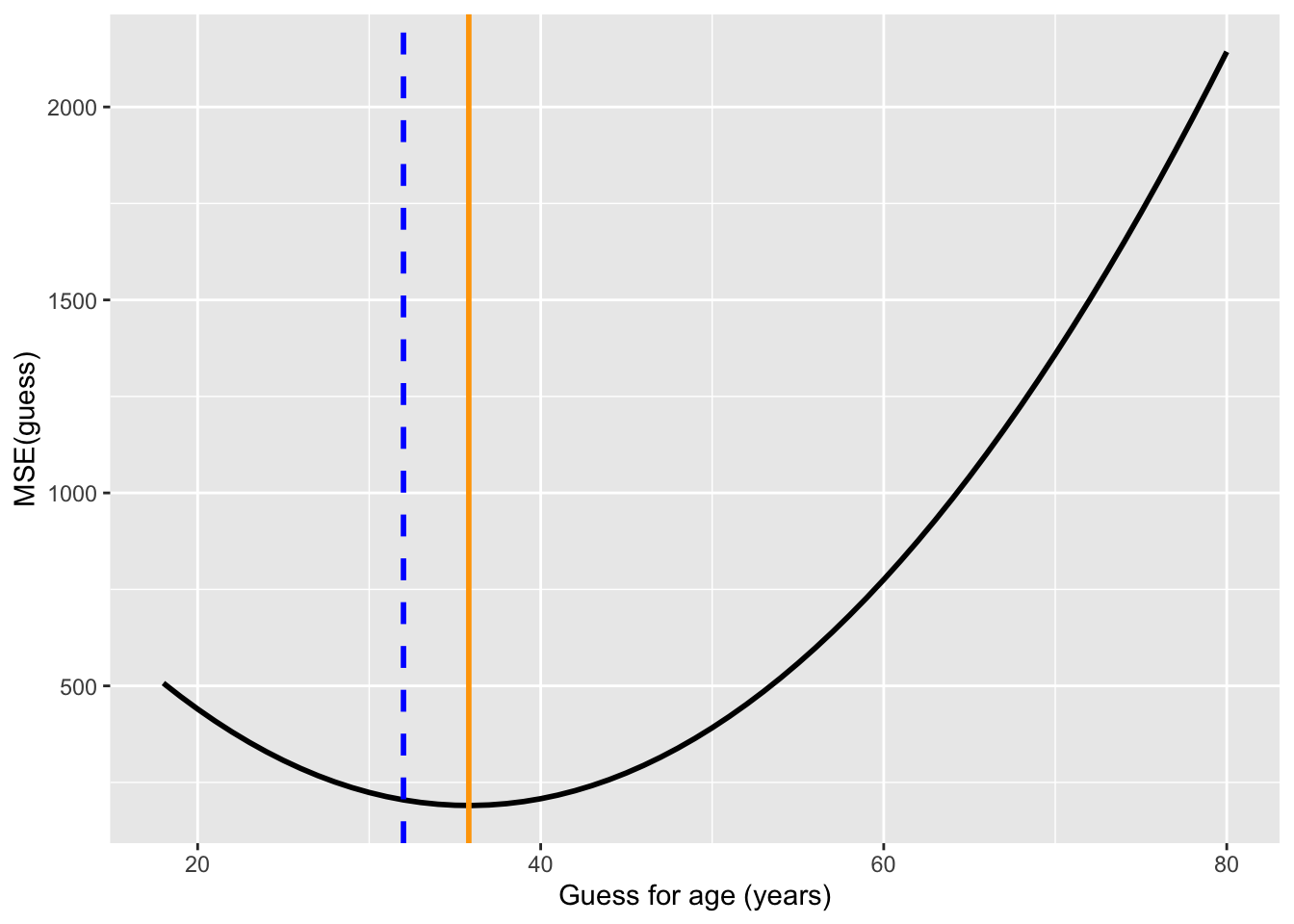
The bowl bottoms out at the mean (35.8, orange), not the median (32, blue dashed). Ages are skewed right: a few older respondents pull the mean above the median, and squaring makes the guess pay close attention to them.
WarningMethods portfolio
- Find the bottom with calculus. Show that the guess that minimizes \(\text{MSE}(g)\) is the mean, \(\bar{Y}\) (and so not the median or the mode). To find the bottom of the bowl, find the value of \(g\) that makes the first derivative of \(\text{MSE}(g)\) equal to zero.
Question 3: The median of the effects isn’t the difference of the medians
In class, we said that the average of the individual effects equals the difference of the averages, which is why we can learn an average effect from two groups. The same isn’t true of the median. Here you’ll check both claims.
The code below makes up commute times for 1,000 people. Everyone has a commute by bike. For 60% of people, the bus takes exactly as long; for the other 40%, it adds 20 minutes.
set.seed(211)
commute = tibble(
  bike = round(rnorm(1000, mean = 25, sd = 8)),               # minutes by bike
  bus_adds = sample(c(0, 20), 1000, replace = TRUE,           # extra minutes by bus:
                    prob = c(0.6, 0.4)),                      #   0 for 60%, 20 for 40%
  bus = bike + bus_adds                                       # minutes by bus
)- Make a new column with each person’s individual effect of taking the bus: their bus time minus their bike time. Compute the average of the individual effects, and the difference of the averages (average bus time minus average bike time). Are they equal?
TipAnswer
commute = commute |>
  mutate(effect = bus - bike)

commute |>
  summarize(average_of_effects = mean(effect),
            difference_of_averages = mean(bus) - mean(bike))
# A tibble: 1 × 2
average_of_effects difference_of_averages
<dbl> <dbl>
1 8.16 8.16They’re equal, and they always will be: adding up everyone’s differences gives the same total as adding up all the bus times and subtracting all the bike times.
- Now do the same with the median: compute the median of the individual effects, and the difference of the medians. Are they equal?
TipAnswer
commute |>
  summarize(median_of_effects = median(effect),
            difference_of_medians = median(bus) - median(bike))
# A tibble: 1 × 2
median_of_effects difference_of_medians
<dbl> <dbl>
1 0 7Not even close. The median person’s commute doesn’t change at all (most people’s effect is 0), but the difference of the medians says the bus adds 7 minutes.
Question 4: Covariance by hand
Here are five made-up observations of two variables:
| Unit | \(X\) | \(Y\) |
|---|---|---|
| 1 | 2 | 3 |
| 2 | 4 | 7 |
| 3 | 6 | 5 |
| 4 | 8 | 11 |
| 5 | 10 | 9 |
- Compute \(\text{Cov}(X, Y)\) by hand (a calculator is fine).
TipAnswer
First the averages: \(\bar{X} = (2 + 4 + 6 + 8 + 10) / 5 = 6\) and \(\bar{Y} = (3 + 7 + 5 + 11 + 9) / 5 = 7\). Then each unit’s two misses and their product:
| Unit | \(X_i - \bar{X}\) | \(Y_i - \bar{Y}\) | Product |
|---|---|---|---|
| 1 | \(-4\) | \(-4\) | 16 |
| 2 | \(-2\) | 0 | 0 |
| 3 | 0 | \(-2\) | 0 |
| 4 | 2 | 4 | 8 |
| 5 | 4 | 2 | 8 |
\(\text{Cov}(X, Y) = (16 + 0 + 0 + 8 + 8) / 5 = 32 / 5 =\) 6.4
Unit 1 is below average on both variables and units 4 and 5 are above average on both, so all three add. Units 2 and 3 sit exactly at the average on one variable, so they add nothing. No unit is above average on one and below on the other, so nothing subtracts.
- Put the data in a tibble and compute the covariance with
cov(). Why isn’t R’s answer the same as yours? (Hint: what did we say in lecture about the denominator R uses?)
TipAnswer
toy = tibble(x = c(2, 4, 6, 8, 10), y = c(3, 7, 5, 11, 9))
cov(toy$x, toy$y)
[1] 8R gives 8, not 6.4. Like sd(), R’s cov() divides by \(n - 1\) instead of \(n\): \(32 / 4 = 8\). As we said in lecture, \(n - 1\) matters when our data are a sample from a bigger population; more on that later in the course.
- Turn your covariance into a correlation, and check your answer with
cor().
TipAnswer
Divide the covariance by the standard deviation of \(X\) times the standard deviation of \(Y\). The squared misses on \(X\) are 16, 4, 0, 4, 16, so \(\text{Var}(X) = 40 / 5 = 8\). On \(Y\) they’re 16, 0, 4, 16, 4, so \(\text{Var}(Y) = 40 / 5 = 8\) too. Then
\[ r = \frac{\text{Cov}(X, Y)}{\text{SD}(X) \, \text{SD}(Y)} = \frac{6.4}{\sqrt{8} \times \sqrt{8}} = \frac{6.4}{8} = 0.8 \]
cor(toy$x, toy$y)[1] 0.8cor() agrees. Dividing by \(n\) or by \(n - 1\) doesn’t matter here, as long as you do the same in the covariance and the SDs: it cancels between the top and the bottom.
Question 5: The average of \(Y\) at each value of \(X\)
county_data (in socviz) has one row for each US county, including the Democratic candidate’s share of the presidential vote in 2012 (per_dem_2012) and 2016 (per_dem_2016). Start with this code, which keeps counties with both and turns the shares into percents:
counties = county_data |>
  filter(!is.na(per_dem_2012), !is.na(per_dem_2016)) |>
  mutate(dem_2012 = 100 * per_dem_2012,
dem_2016 = 100 * per_dem_2016)- Make a scatterplot with the 2012 vote on the x-axis and the 2016 vote on the y-axis. Describe the relationship’s direction and strength.
TipAnswer
ggplot(counties, aes(x = dem_2012, y = dem_2016)) +
  geom_point(alpha = 0.2) +
  labs(x = "Democrat's % of the vote, 2012", y = "Democrat's % of the vote, 2016")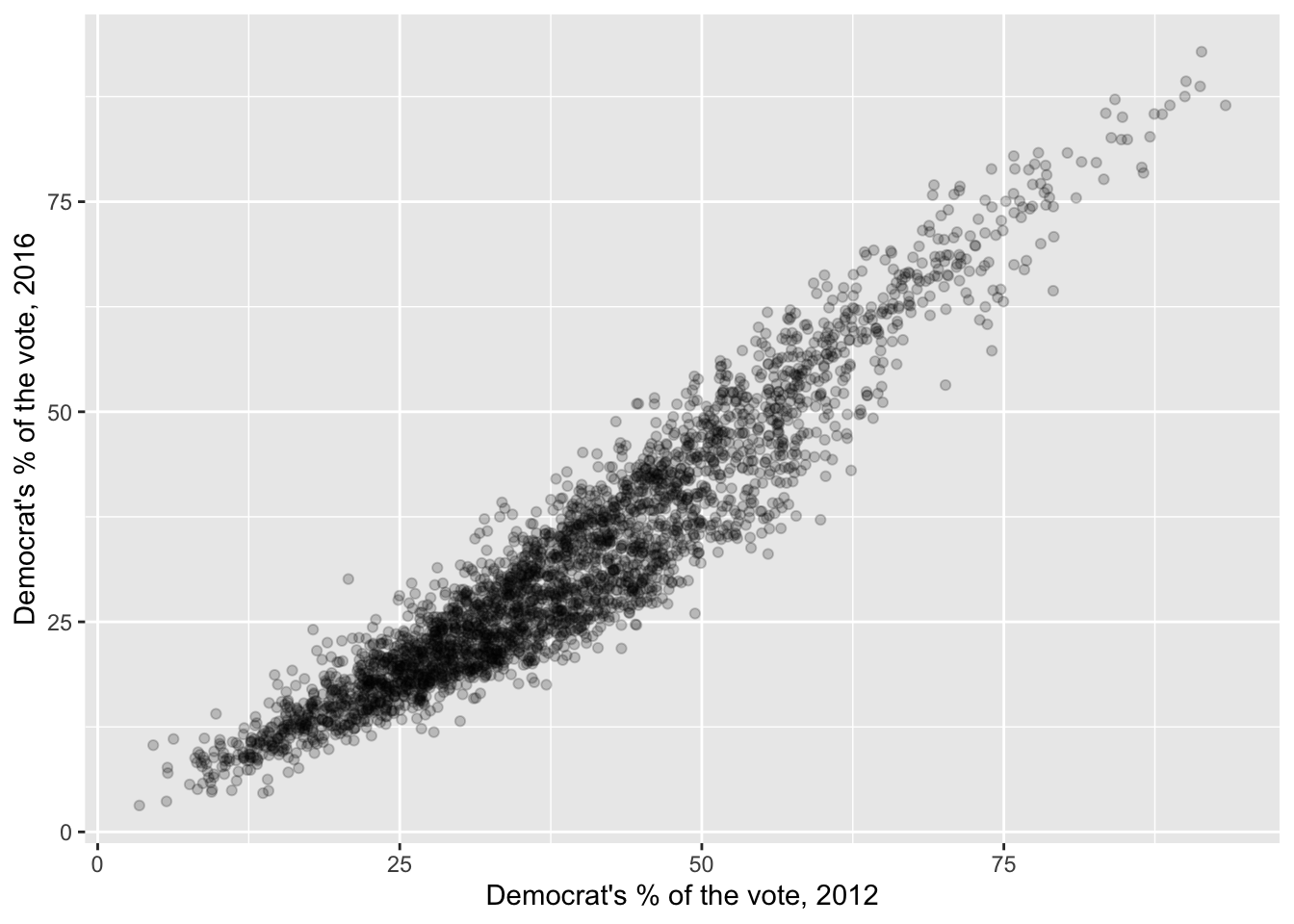
Positive and very strong: counties that voted more Democratic in 2012 did so again in 2016, and the points hug a line tightly (cor() gives 0.95).
- Estimate \(E[\text{2016 vote} \mid \text{2012 vote}]\) with bins.
ntile(x, 10)sorts the values ofxand splits them into 10 bins with equal numbers of counties: 1 for the lowest tenth, 10 for the highest. Add a bin column, then, for each bin, compute the average 2012 vote, the average 2016 vote, and the number of counties.
TipAnswer
bins = counties |>
  mutate(bin = ntile(dem_2012, 10)) |>
  group_by(bin) |>
  summarize(dem_2012 = mean(dem_2012),
            dem_2016 = mean(dem_2016),
            counties = n())

bins
# A tibble: 10 × 4
bin dem_2012 dem_2016 counties
<int> <dbl> <dbl> <int>
1 1 15.6 12.3 312
2 2 23.5 17.9 312
3 3 27.8 20.9 311
4 4 31.6 23.9 311
5 5 35.3 27.3 311
6 6 39.1 30.7 311
7 7 43.2 34.2 311
8 8 47.7 39.5 311
9 9 54.2 47.1 311
10 10 67.2 63.2 311Each row is a conditional mean: the average 2016 vote among counties in one slice of the 2012 vote.
- Add the bin averages to your scatterplot as large points (a second
geom_point()withdata = bins). Do they follow the cloud?
TipAnswer
ggplot(counties, aes(x = dem_2012, y = dem_2016)) +
  geom_point(alpha = 0.1) +
  geom_point(data = bins, color = "orange", size = 4) +
  labs(x = "Democrat's % of the vote, 2012", y = "Democrat's % of the vote, 2016")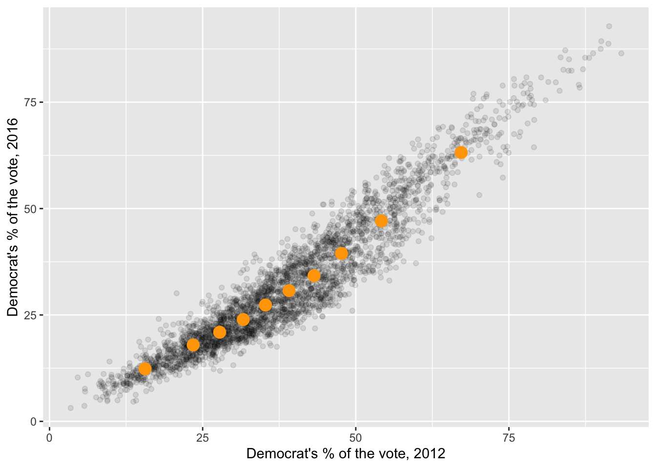
They run right through the middle of the cloud: each one is the average height of the counties in its slice.
- Redo (b) and (c) with 3 bins and with 50 bins. What do you gain and lose with more bins?
TipAnswer
map(c(3, 50), \(k) counties |>
      mutate(bin = ntile(dem_2012, k)) |>
      group_by(bin) |>
      summarize(dem_2012 = mean(dem_2012), dem_2016 = mean(dem_2016)) |>
      mutate(bins = paste(k, "bins"))) |>
  list_rbind() |>
  ggplot(aes(x = dem_2012, y = dem_2016)) +
  geom_point(data = counties, alpha = 0.05) +
  geom_point(color = "orange", size = 2.5) +
  facet_wrap(~bins) +
  labs(x = "Democrat's % of the vote, 2012", y = "Democrat's % of the vote, 2016")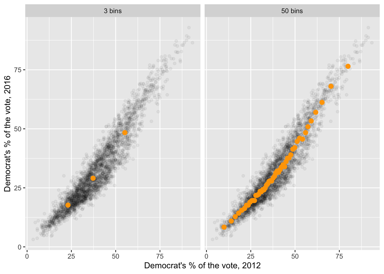
With 3 bins, each average rests on more than 1,000 counties, so it’s very stable, but it smears together very different counties and misses the shape. With 50 bins, the averages trace the relationship closely, but each rests on only about 60 counties, so they’re noisier. More bins: more detail, more noise. With 3,000 counties there’s room for many bins; with 100 there wouldn’t be.