Recap: an estimate is one draw from a sampling distribution
Week 7: a good estimator is centered on the truth (unbiased), tight (small variance), and closes in as \(n\) grows (consistent)
Recap: 95% of studies land within 1.96 standard errors of the truth
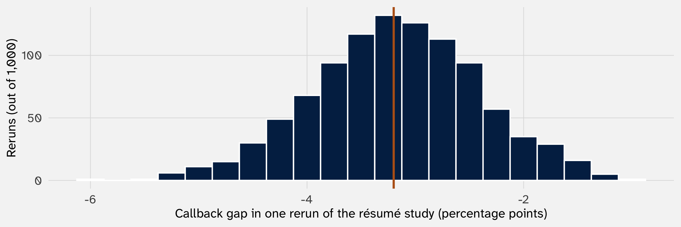
Week 6: centered on the truth, a standard error of 0.78 points, and a Normal distribution. So 95% of studies land within \(1.96 \times\) 0.78 \(\approx\) 1.5 points of the truth
Remember: if the sampling distribution wasn’t Normal, we couldn’t say this!
Recap: the standard error is itself an estimate
The standard error’s formula needs the true callback chances. We only have \(\hat{p}\), so we plug it in:
Week 6: the law of large numbers is why this works. With thousands of résumés, \(\widehat{SE}\) lands close to the true width
Recap: we only have the one study
What can we say from our one study about what estimates from other studies would produce?
We are going to take our onepoint estimate, its estimatedstandard error, and produce a (95%) confidence interval
Today: two questions
1. What is a 95% confidence interval, exactly?
Building one from the sampling distribution
What “95%” means + two tempting readings that are wrong
Why 95%, and getting the 95% right for small samples: the \(t\) distribution and the CLT
2. How can we use a confidence interval?
Identify which values the data can’t rule out
Compare two estimates; are they different?
Plan a study, read R’s output, and know what’s being rerun
What is a 95% confidence interval, exactly?
An interval catches the truth whenever its estimate lands close to the truth
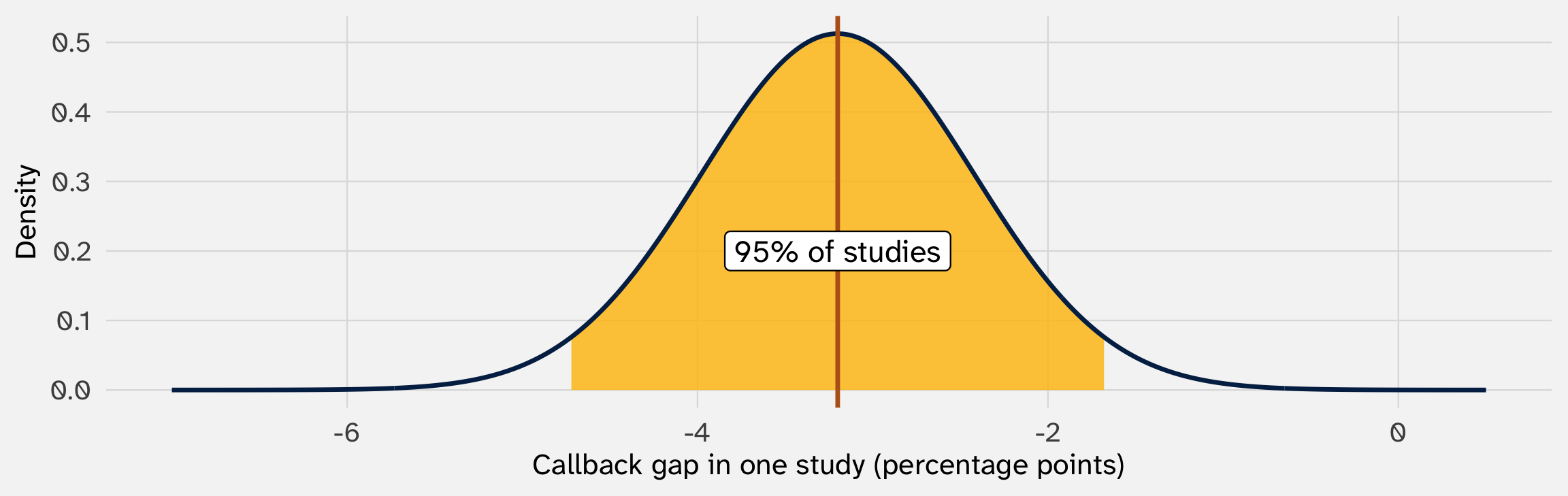
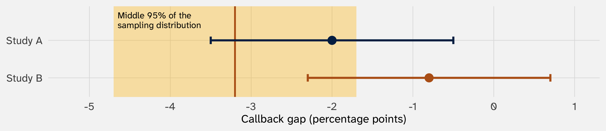
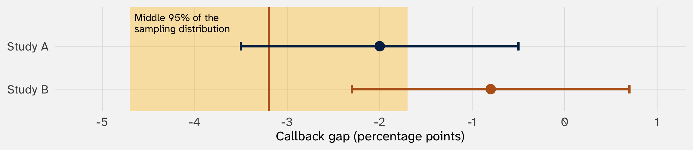
Truth: −3.2. SE: 0.78, so \(1.96 \times SE \approx 1.5\). The gold band is the middle 95% of the sampling distribution, truth ± 1.5: where 95% of studies land (week 6)
Study A got −2.0: 1.2 points from the truth, inside the gold band. So the truth is 1.2 points from −2.0, and \(-2.0 \pm 1.5 = [-3.5, -0.5]\)catches −3.2
Study B got −0.8: 2.4 points off, one of the unlucky 5%. Its interval, \([-2.3, 0.7]\), misses
How many studies will cover the truth?
The 95% confidence interval:
if an estimate lands in the gold band, then \(\text{estimate} \pm 1.96 \times \widehat{SE}\) catches the truth
95% of studies will land in the gold band (i.e., within 1.96 SE of the truth)
Notice! 95% of confidence intervals cover the truth; no clue whether yours does or not (and that’s OK)
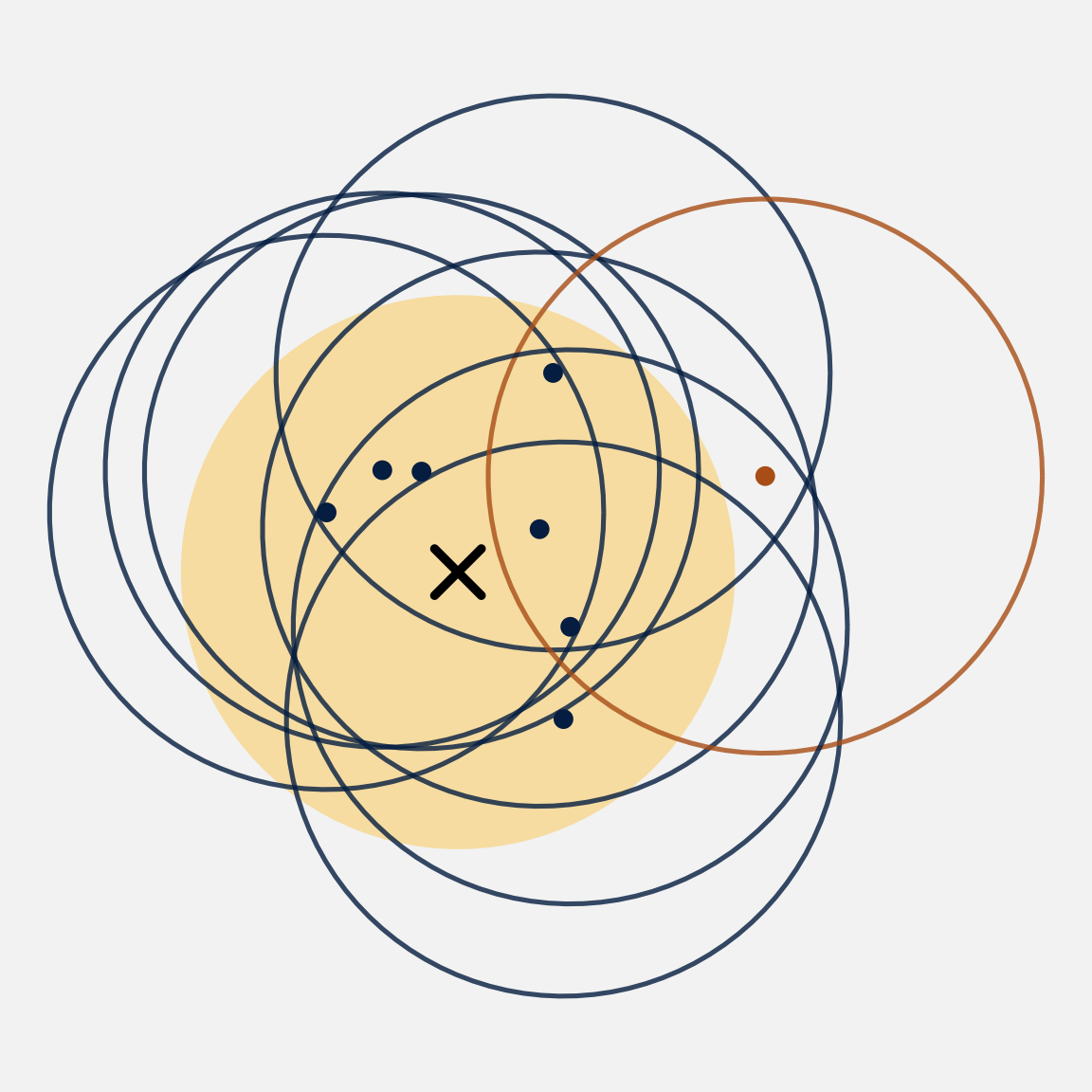
Same idea on a dartboard: a hoop around each dart
The bullseye (✕) is the truth. 95% of darts land inside the gold circle
Around each dart, draw a hoop the same size as the gold circle: that’s the interval
Dart inside the gold circle: its hoop covers the bullseye (blue)
Dart outside: its hoop misses (orange)
So 95% of hoops cover the bullseye. But in one study you see your dart and your hoop, never the bullseye
The same argument, in symbols
Remember: if we standardize the estimate, we get a standard normal (week 6):
Read it carefully. What’s random here is the interval. Its endpoints, \(\hat{\Delta} \pm 1.96 \, SE\), are built from the point estimate \(\hat{\Delta}\), which changes from study to study. \(\Delta\), the truth, is a fixed number (for now, treat the \(SE\) as fixed too; the \(t\) section relaxes that)
We built it with the recipe estimate ± 1.96 SE, which catches the truth in 95% of studies
But did our interval catch the true gap? From one study, we can’t tell
One rerun of the study, one interval
Week 4’s résumé DGP, with a true gap of −3.2 points. Run it once, and build the interval exactly as we did for the real data:
set.seed(211)one_run =gap_and_se() |># one rerun: 4,870 new résumés, the gap, its SEmutate(lower = gap -1.96* se, # the 95% intervalupper = gap +1.96* se)
One simulated rerun of the résumé study, in percentage points. Made-up data from week 4’s DGP.
Gap
SE
Lower
Upper
Contains −3.2?
-2.02
0.77
-3.53
-0.52
Yes
This rerun’s estimate is -2.0, more than a point off. But its interval reaches back to −3.2: it catches the truth
Ten reruns, ten intervals
The first 10 of 1,000 simulated reruns of the résumé study, in percentage points. Made-up data from week 4’s DGP.
Rerun
Gap
SE
95% interval
Contains −3.2?
1
-2.02
0.77
[-3.53, -0.52]
Yes
2
-3.54
0.75
[-5.02, -2.07]
Yes
3
-1.68
0.77
[-3.20, -0.17]
Yes
4
-3.05
0.77
[-4.57, -1.54]
Yes
5
-3.21
0.76
[-4.69, -1.73]
Yes
6
-2.76
0.78
[-4.28, -1.24]
Yes
7
-3.02
0.78
[-4.54, -1.50]
Yes
8
-2.22
0.78
[-3.76, -0.68]
Yes
9
-3.94
0.79
[-5.50, -2.39]
Yes
10
-2.82
0.79
[-4.36, -1.28]
Yes
Every rerun gets its own estimate and its own SE (it’s estimated each time), so its own interval. All 10 catch the truth; rerun 3 only just (its interval starts at -3.20)
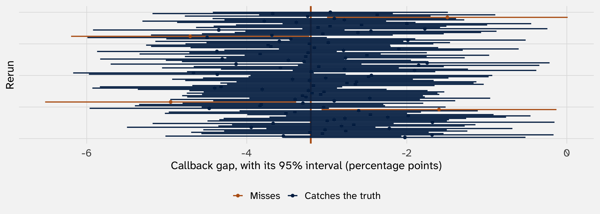
Rerun the study 100 times: 100 intervals
96 of these 100 contain the true gap (orange line); over all 1,000 reruns, 95.2%. That share is the interval’s coverage: the share of reruns whose interval contains the truth. A 95% interval should have 95% coverage
The right reading: 95% describes the method, not this interval
Coverage: across many studies, 95% of intervals built this way contain the truth
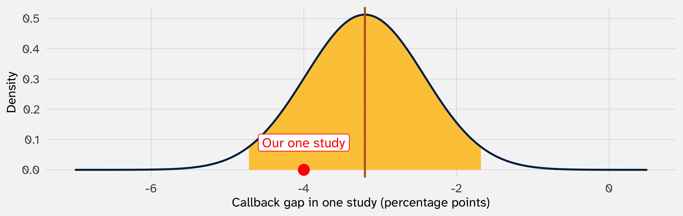
One interval either contains the truth or it doesn’t. We don’t know which. Our \([-4.7, -1.7]\) is one of the 1,000 lines on the last slide
So the careful (brutally awkward) sentence is: “Our 95% confidence interval, -4.7 to -1.7 points, came from a method that catches the true gap in 95% of studies”
Our one interval
What can we say then about our study’s interval -4.7 to -1.7?
✅ “A good bet”: with no other information, betting that the true gap is between −4.7 and −1.7 is reasonable. Bets made this way win in 95% of studies
❌ “There’s a 95% chance this bet wins”: this one bet is already won or lost; we just can’t see which (the covered coin, next slide)
The 95% is about the method; the bounds are about our data
A kitchen scale reads within 1 gram of the true weight 95% of the time. You weigh coffee beans: it reads 18. So you say the beans weigh 17 to 19 grams. The rule “reading ± 1” is right 95% of the time; this time it says 17 to 19
Our \([-4.7, -1.7]\) works the same way. Different data would give different bounds, so these bounds tell us something:
Which gaps fit our data: every gap inside does; zero, far outside, doesn’t (Part 2)
How precise the study is: 3.1 points wide. With 500 résumés, it would be about 10 points wide (Part 2)
A rule to act on: treat the true gap as inside the interval. Follow that rule in every study, and you’ll be right in 95% of them. That’s a track record for the rule
The one thing the bounds can’t give you: “a 95% chance the true gap is in \([-4.7, -1.7]\)”
A covered coin: the probability belongs to the rule, not the guess
Flip a fair coin. Before it lands: a 50% chance of heads
Now it’s landed, under your hand. It’s heads or tails, already decided. Two ways to talk about it:
Method 1: “If you always guess heads, you’re right half the time.” A track record for the rule
Method 2: “There’s a 50% chance it’s heads.” A probability about this coin (more on this view soon)
Our interval is the covered coin. Before the study: a 95% chance the interval will catch the true gap. After: it’s \([-4.7, -1.7]\), and it either caught it or didn’t. Always acting as if it did makes you right in 95% of studies
Why is this so tortured? Frequentist vs. Bayesian interpretations
What’s the difference, exactly? Why can’t we say there’s a 95% chance the true gap is in the interval?
✅ “Bets made this way win in 95% of studies”
❌ “There’s a 95% chance this bet wins”
“95% probability the truth is in this interval” treats the truth as random. In the statistics we’ve done all term (frequentist), the truth is a fixed number; probability describes procedures: what happens across reruns
There is a way to make that second statement: using Bayesian statistics, in which probability describes beliefs how about how likely an event is
Bayesian credible intervals
Bayesian statistics gives the parameter its own probability distribution:
A prior distribution: what you believe about \(\Delta\) before the data (e.g., the gap could be anywhere from -10 to +10)
The data update it, by Bayes’ rule, into a posterior distribution: what you believe after
A 95% credible interval holds 95% of the posterior. For that interval, “a 95% probability the truth is in here” is the right reading
The Bayesian credible interval is the more intuitive (yet forbidden) claim we wish to make with our confidence interval
When does the credible interval == the confidence interval?
With a lot of data and a flat prior (no strong beliefs beforehand), the 95% credible interval and the 95% confidence interval will be roughly equal. Why is this helpful?
It means there’s a world where you could say that there’s a 95% probability that the true callback gap is between -4.7 and -1.7 points; when you have no prior beliefs about the size of the gap
This is why the Bayesian reading of a confidence interval is so common, and often harmless in practice
Which to use? A debate older than this field. This course is frequentist, as are most papers you’ll read. Say “95% confidence,” and mean “a method that works 95% of the time” (Greenland et al. 2016)
Your turn: what does \([1, 9]\) mean?
A get-out-the-vote study finds an effect on turnout of 5 points
Its standard error is 2 points
By hand: the 95% confidence interval (use 2 in place of 1.96)
Which of these are right?
“There’s a 95% probability that the true effect is between 1 and 9 points”
“The interval \([1, 9]\) came from a method that catches the true effect in 95% of studies”
“95% of studies like this one would find an effect between 1 and 9 points”
“Betting that the true effect is between 1 and 9 points is a sensible bet: the method behind it wins in 95% of studies”
What does \([1, 9]\) mean? Answers
1.\(5 \pm 2 \times 2 = [1, 9]\)
2.
(a) Wrong, as a frequentist statement: the true effect isn’t random; it’s in \([1, 9]\) or it isn’t. (It’s the right reading of a Bayesian interval: coming up)
(b) Right: the 95% describes the method that produced \([1, 9]\), not \([1, 9]\) itself
(c) Wrong: 95% of studies land within 2 SEs of the truth, not of our estimate. If the truth were 2, most studies would land between −2 and 6. More on the next slide
(d) Right: the bet is about \([1, 9]\) itself, and the 95% stays with the method. With no other information, treating this study as a typical draw from the method’s track record is fair. (Know something else, like other studies’ results? Then the fair odds can change)
A 95% interval is not a forecast of the next study
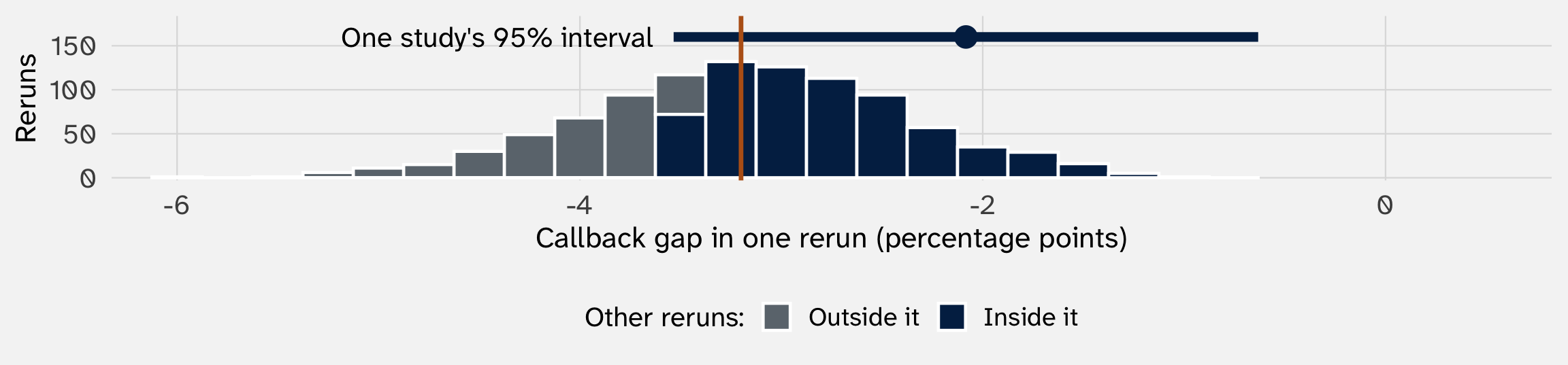
Answer (c) treated the interval as a forecast. Check: one rerun’s interval against the other 999 reruns
This interval holds only 68% of the other reruns (its estimate landed a bit high). Averaged over all 1,000 intervals: 83%, not 95% (Cumming and Maillardet 2006)
Why it matters: a replication that lands outside the original interval is often called a failure. Even when nothing is wrong, that happens about 1 time in 6
Why 95%?
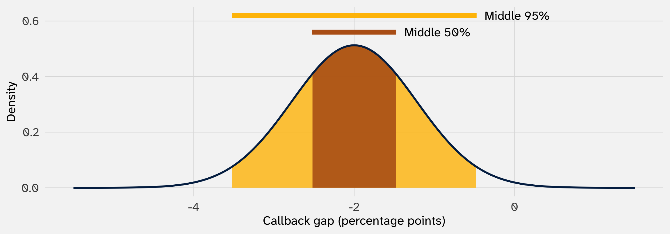
Any middle share of the bell makes an interval. Which share?
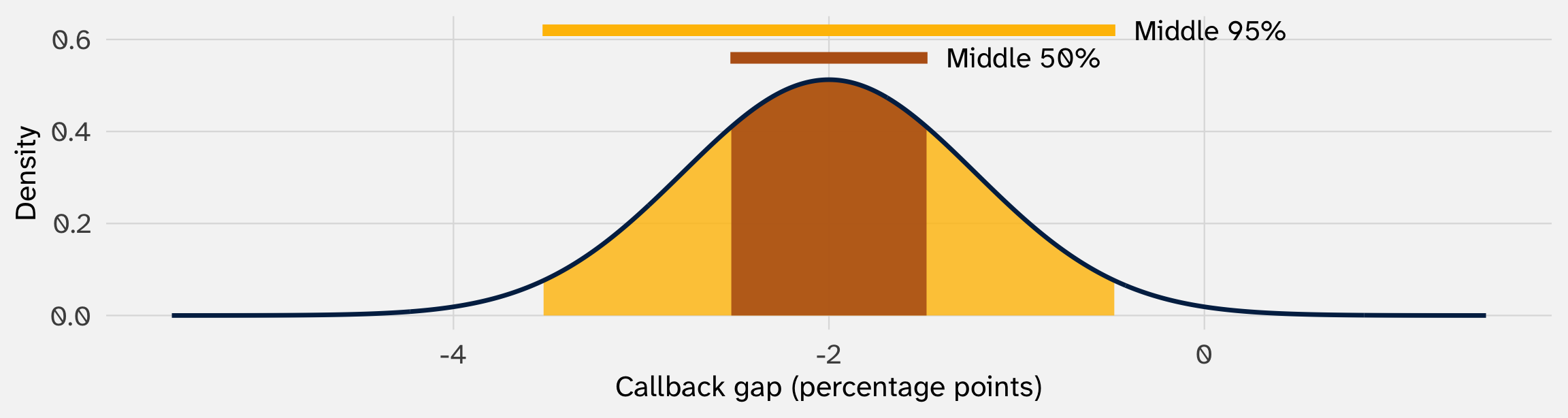
Say a study got −2, with a standard error of 0.78. Draw a bell around its estimate, with SD = the standard error. Report where the middle 50% falls (orange)? The middle 95% (gold)?
The tradeoff: a narrower interval, less confidence
50% interval: [-2.5, -1.5] points. Narrow, but it misses the truth in half of studies
95% interval: [-3.5, -0.5] points. Wider, and it misses in only 1 in 20
A narrower interval is more informative but is more likely to miss the truth
Where the 1.96 comes from, and other levels’ multipliers
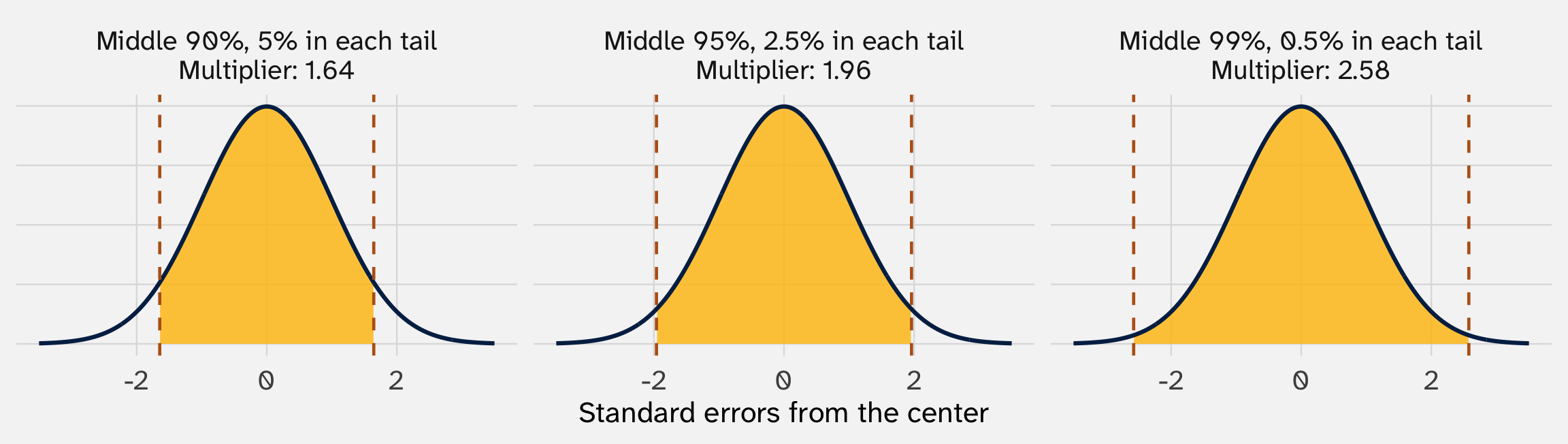
The 1.96 is where the middle 95% of a standard normal ends: 2.5% is left over in each tail. For a 90% interval, find where the middle 90% ends: 1.64. For 99%: 2.58
Other levels: swap the 1.96
Statisticians call the leftover share \(\alpha\) (“alpha”). For a 95% interval, \(\alpha = 5\%\): 2.5% in each tail
So the multiplier for any level is qnorm(1 - alpha / 2). For 95%: qnorm(1 - 0.05 / 2) = qnorm(0.975) = 1.96
Each level’s multiplier, and the résumé study’s interval at that level. Data: resume.csv.
Confidence level
Multiplier, z
Résumé gap interval (points)
80%
1.282
[-4.2, -2.2]
90%
1.645
[-4.5, -1.9]
95%
1.960
[-4.7, -1.7]
99%
2.576
[-5.2, -1.2]
Convention is 95%, and it’s only a convention. 100% confidence is easy, and useless: \((-\infty, \infty)\)
Let’s take a 10-minute break
Does our “95%” really cover 95%? Two assumptions
Every interval so far: estimate ± multiplier × SE, with the multiplier read off a normal bell (1.96 for 95%)
That recipe assumes two things:
We know the SE. We don’t: we estimate it from the same data. With 4,870 résumés the estimate is close (the ten reruns: 0.75 to 0.79). With 5 observations, it’s noisy
The sampling distribution is Normal. The CLT promises that for large samples. For small samples of skewed data, not quite
If either fails, a “95%” interval catches the truth less than 95% of the time. Next: how much less, and the fix for each
Doesn’t this all depend on \(\sigma\) being known?
Say we canvass \(n\) voters, and each answer is a draw from a normal population, \(N(\mu, \sigma^2)\) (week 6’s canvass: \(\mu = 40\), \(\sigma = 20\)). If we knew \(\sigma\):
\[
Z = \frac{\bar{Y} - \mu}{\sigma / \sqrt{n}} \sim N(0, 1)
\qquad \Rightarrow \qquad
\bar{Y} \pm 1.96 \, \frac{\sigma}{\sqrt{n}} \text{ is a 95\% interval}
\]
But we never know \(\sigma\). We estimate it with the sample SD (week 7: divide by \(n - 1\)):
Student’s \(t\) distribution with \(n - 1\)degrees of freedom(Xu 2026)
\(T\) is the t-value: the estimate’s distance from the truth, in estimated standard errors
Its distribution is the same whatever \(\mu\) and \(\sigma\) are: subtracting \(\mu\) removes the center, and dividing by \(S/\sqrt{n}\) removes the spread. So it works like the standard normal: find its middle 95%, and build an interval
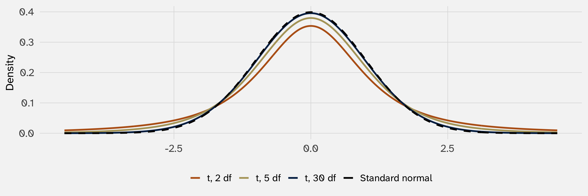
The \(t\) is a bell with heavier tails
heavier tails: an estimated SE is sometimes too small, so big t-values happen more often. As \(n\) grows, \(S\) settles on \(\sigma\) (the LLN) and the \(t\) becomes the normal
Heavier tails mean a bigger multiplier
A 95% interval with an estimated SE: \(\bar{Y} \pm t_{n-1} \times S / \sqrt{n}\), with the multiplier from qt(0.975, df = n - 1)
Sample size, \(n\)
Degrees of freedom
95% multiplier
3
2
4.30
5
4
2.78
10
9
2.26
30
29
2.05
100
99
1.98
1,000
999
1.96
Normal (n very large)
1.96
With 5 observations the multiplier is 2.78, not 1.96. By 100, the difference is negligible
Check it: 1.96 with an estimated SE undercovers when \(n\) is small
A normal population (the canvass noise from week 6: mean 40, SD 20). Draw samples, plug in \(S\), and build intervals two ways. 10,000 reruns each
10,000 simulated samples at each size. Made-up data.
Sample size
Coverage with 1.96
Coverage with the t multiplier
5
87.6%
94.7%
30
94.2%
95.2%
With 5 observations, “± 1.96 estimated SEs” catches the truth only 88% of the time: the advertised 95% is a lie. The \(t\) multiplier fixes it. With 30, the two barely differ
Any population, large \(n\): the interval works anyway
The \(t\) theorem assumed a normal population. For any population with a finite variance, the CLT says \(\bar{Y}\) is about normal for large \(n\), and \(S \rightarrow \sigma\) (the LLN), so
\[
\bar{Y} \pm t_{n-1} \frac{S}{\sqrt{n}} \text{ has coverage close to 95\%}
\]
Week 7’s skewed protest population, 10,000 simulated samples at each size. Made-up data.
Sample size
Coverage of the t interval
5
93.6%
30
94.1%
200
95.0%
Skewed data, small \(n\): a little short of 95%. By a few hundred, right on
The résumé study is this case: callbacks are 0 or 1, nothing like a normal. With 4,870 résumés, the CLT overwhelms. Our rerun coverage: 95.2%
How can we use a 95% confidence interval?
In practice: the interval holds the values the data can’t rule out
Strictly, 95% describes the method. But there’s a second, practical reading of one interval:
If the true gap were any value inside \([-4.7, -1.7]\), our estimate would be an ordinary result: inside the middle 95% of where studies land. If it were any value outside, our estimate would be a fluke
So the interval is the range of gaps compatible with the data. Values outside it, zero included, are hard to square with what we saw. Week 9 shows why the two readings line up
Using the résumé interval
Direction is settled. Zero is outside the interval, and so is any (positive) gap that favors AA-named résumés
The low end rules out “tiny.” The gap is at least 1.7 points: about 17% fewer callbacks than white-named résumés’ 9.7%
The high end rules out “huge.” The gap is at most 4.7 points: about 49% fewer. A claim that AA-named résumés get, say, a third of the callbacks isn’t supported
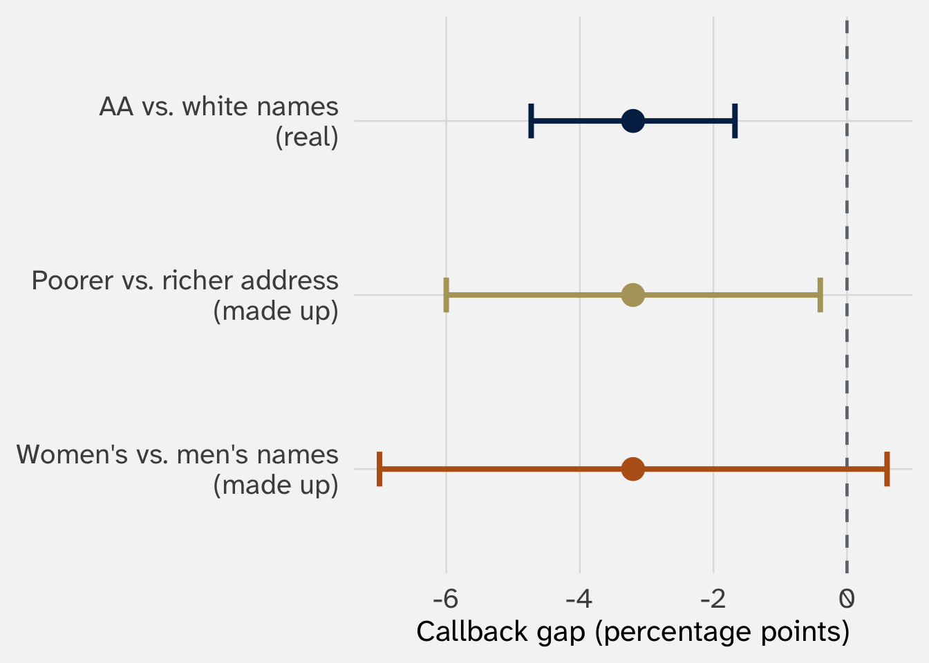
Same estimate, different widths: how much did we learn?
All three estimate a gap of -3.2 points
Race (narrow): the gap is between 1.7 and 4.7 points. Direction settled, size pinned down
Address (wide): direction settled, size not: the gap could be trivial (0.4) or huge (6)
Gender (crosses zero): the data fit a penalty, no gap, or a small boost. Not evidence of no effect (more next week): we just can’t tell
Two intervals overlap. Is there a difference?
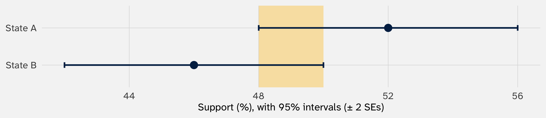
Support for a policy is 52% in state A and 46% in state B. Is the policy more popular in state A?
The intervals, \([48, 56]\) and \([42, 50]\), overlap (shaded). Tempting conclusion: “no clear difference in popularity across states”
The interval for the difference excludes zero
The difference is \(52 - 46 = 6\) points. Its standard error (week 5’s difference rule, independent samples):
Read both ends of each interval. What does each one tell you?
Why is one interval so much wider than the other?
Is the race gap different for women’s and men’s names? (Don’t eyeball the overlap)
Women’s and men’s names: answers
The race gap in callbacks, by the name’s sex. Data: resume.csv.
Names
Résumés
Gap (points)
95% interval
Women’s
3,746
-3.3
[-5.0, -1.5]
Men’s
1,124
-3.0
[-6.1, 0.0]
Difference (women − men)
-0.2
[-3.7, 3.3]
Women’s: the sign is settled; the gap is 1.5 to 5.0 points. Men’s: about the same estimate, but the interval runs right up to zero
Width: about a third as many men’s résumés, so a bigger SE. The real-data version of “same estimate, different widths”
We can’t tell. The difference’s interval, \([-3.7, 3.3]\), includes zero. That’s not evidence the gaps are equal: the data fit a gap for men up to 3.7 points bigger or smaller
Use confidence intervals for planning
Say we run our own résumé study, with a racial marker as the treatment. The original found a gap of -3.2 points, ± 1.5 with 4,870 résumés. How many résumés do we need?
Margins of error at each sample size, if our study found the original’s gap and callback rates. Based on resume.csv.
Résumés
Margin of error
Interval, if we found −3.2
What we’d learn
500
± 4.8
[-8.0, 1.6]
Useless: crosses zero, sign unknown
1,000
± 3.4
[-6.6, 0.2]
Useless: crosses zero, sign unknown
2,000
± 2.4
[-5.6, -0.8]
Sign settled, size rough
4,870
± 1.5
[-4.7, -1.7]
The original study
20,000
± 0.8
[-4.0, -2.5]
Very precise: maybe overkill
45,000
± 0.5
[-3.7, -2.7]
Very precise: maybe overkill
To halve the margin, you need four times the résumés. Decide how precise you need to be, then pick the smallest study that gets there (Lakens 2022)
R does all of this for you
lm(call ~I(race =="black"), data = resume) |>confint()
The second row: -4.7 to -1.7 points, the interval we built by hand (lm() uses the \(t\) multiplier, which with 4,868 degrees of freedom is 1.96)
Week 1’s table said −0.032 (0.0078). Now every piece has a meaning:
−3.2 points: the estimate, one draw from a sampling distribution centered on the true gap (weeks 4 and 5)
0.78 points: its standard error, estimated from one run of data (weeks 5 and 6)
[−4.7, −1.7]: an interval from a method that catches the true gap in 95% of studies (today)
What if our data are the whole population?
A confidence interval’s 95% is about reruns. With all 50 states, or every country, nobody was sampled. What gets rerun?
Describing these 50 states? Then nothing is random. The difference in means is just a fact about them, and there’s no standard error (Wooldridge 2023, 3)
Learning about the process that made them? Then the 50 states are one run of a process that could have come out differently (week 4: rerun the French Revolution). The standard error says how much the estimate would change across runs
Most political science asks the second question, so papers report standard errors even with all-country data (Abadie et al. 2020)
In an experiment, the standard error makes sense even with everyone
Say the résumé study had covered every employer in Boston and Chicago. Is anything still random?
Yes: which résumés got which names. Each employer saw only one version of each résumé (week 1). Flip the coins again, and the estimate changes
So for a difference in means, the usual standard error still works: it’s right, or a little too big. It breaks down for purely descriptive facts about the units we have, and when draws come in clusters (week 10)
Next week: testing
An interval asks: which values of the truth fit the data?
A test asks the flip side: does one particular value, like zero, fit the data? Week 9: hypothesis tests, p-values, and Bayes’ rule, to read a p-value the right way
We will see that a 95% interval that excludes zero is the same as a test that rejects zero at the 5% level
References
Abadie, Alberto, Susan Athey, Guido W. Imbens, and Jeffrey M. Wooldridge. 2020. “Sampling-Based Versus Design-Based Uncertainty in Regression Analysis.”Econometrica 88(1): 265–96. doi:10.3982/ECTA12675.
Cumming, Geoff, and Robert Maillardet. 2006. “Confidence Intervals and Replication: Where Will the Next Mean Fall?”Psychological Methods 11(3): 217–27. doi:10.1037/1082-989X.11.3.217.
Greenland, Sander, Stephen J. Senn, Kenneth J. Rothman, John B. Carlin, Charles Poole, Steven N. Goodman, and Douglas G. Altman. 2016. “Statistical Tests, P Values, Confidence Intervals, and Power: A Guide to Misinterpretations.”European Journal of Epidemiology 31(4): 337–50. doi:10.1007/s10654-016-0149-3.
Lakens, Daniël. 2022. Improving Your Statistical Inferences. doi:10.5281/zenodo.6409077.
Schenker, Nathaniel, and Jane F. Gentleman. 2001. “On Judging the Significance of Differences by Examining the Overlap Between Confidence Intervals.”The American Statistician 55(3): 182–86. doi:10.1198/000313001317097960.
Wooldridge, Jeffrey M. 2023. “What Is a Standard Error? (And How Should We Compute It?).”Journal of Econometrics 237: 105517. doi:10.1016/j.jeconom.2023.105517.