Which estimator should we use?
POL 211 · Week 7
Juan F. Tellez
University of California, Davis
November 10, 2026
Exam 2
Write your answers in your blue book
Let’s take a 10-minute break
Today
- Four candidate estimators of the population average: how do we choose among them?
- Finite-sample properties (true at any \(n\)): unbiased, efficient, and mean squared error
- Asymptotic properties (what happens as \(n\) grows): consistent
- When is the obvious estimator less obvious? Counting the dead
Where we are
All term we’ve estimated with an average. Is that the best way?
Every estimate so far has been an average of something (difference in means, difference in proportions). Is this the best estimator in these situations? How could we know?
“But didn’t week 1 already say why? The average effect equals the difference of the averages.”
That settles what we’re estimating (the estimand). It doesn’t settle how to estimate each average from a sample. An estimator is a rule applied to data; other rules could try to hit the same target
Today: a set of candidate rules (estimators) for the same population average. How do we choose among them? How do we know the sample average is a good estimator?
Qualities of estimators
| Property | What it means | |
|---|---|---|
| Finite-sample: true at any sample size | Unbiased | The sampling distribution is centered on the estimand |
| Efficient | Among unbiased estimators, the one with the smallest spread | |
| Asymptotic: what happens as \(n\) grows | Consistent | The estimator closes in on the estimand (week 6’s law of large numbers) |
| Asymptotically normal | The sampling distribution is a bell once \(n\) is large (week 6’s central limit theorem) |
Four estimators of one average
The average number of protests, per week
Take a minute: why would a researcher want this number?
- A baseline: is this week’s 15 protests unusual, or just a bad week?
- A comparison: a difference in averages across cities, or before and after a policy, is how we estimate effects (week 1)
- Planning: how many officers or monitors a city needs on a typical week
In each case we want the average of a population of weeks, and we only get to see some of them
The estimand: the average number of protests per week
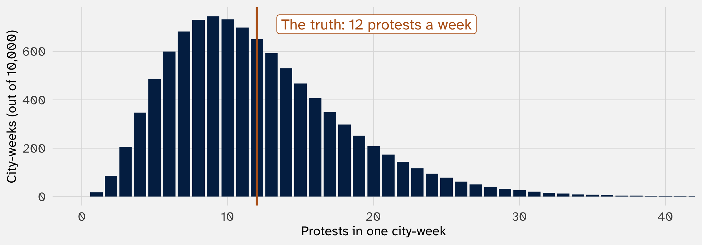
A population of 10,000 city-weeks. We want the average, \(\mu\), but we’ll only see 20 randomly drawn weeks
Four candidate estimators of the average. How do we choose?
| Estimator | Rule | In words | |
|---|---|---|---|
| 1 | \(\hat{\mu}_1\) | \(Y_1\) | The first week only |
| 2 | \(\hat{\mu}_2\) | \(2\) | Ignore the data: always say 2 |
| 3 | \(\hat{\mu}_3\) | \(\bar{Y} = (Y_1 + \cdots + Y_n) / n\) | The sample average |
| 4 | \(\hat{\mu}_4\) | \((Y_1 + \cdots + Y_n) / (n + 5)\) | An “adjusted” average: add up the weeks, but divide by 5 too many |
Adapted from Xu (2026)
Isn’t the sample average the obvious choice?
The estimand is an average, so shouldn’t the estimator be an average, too? Yes, and today shows why
But remember this class isn’t about “sounds right”; it’s about the mathematical foundations of these choices. We need to prove it, and so we need criteria to decide
And for other quantities the obvious rule isn’t always the good one. We’ll end with an example!
Same data in, four different answers out
set.seed(211)

# define function
four = function(y) {                               # y: the weeks we sampled
  tibble(estimator = c("First week", "Always say 2", "Sample average", "Sum ÷ (n + 5)"),
         estimate = c(y[1],                        # 1. the first value in the sample
                      2,                           # 2. ignore the data
                      mean(y),                     # 3. add up, divide by n
                      sum(y) / (length(y) + 5)))   # 4. add up, divide by n + 5
}

# one run
one_sample = sample(protests, size = 20, replace = TRUE)   # 20 weeks, drawn at random
four(one_sample)
# A tibble: 4 × 2
estimator estimate
<chr> <dbl>
1 First week 9
2 Always say 2 2
3 Sample average 10.4
4 Sum ÷ (n + 5) 8.32The truth is 12. One sample can’t tell us which rule is best. We need to know what each rule does across many samples
Rerun the study: each estimator has its own sampling distribution
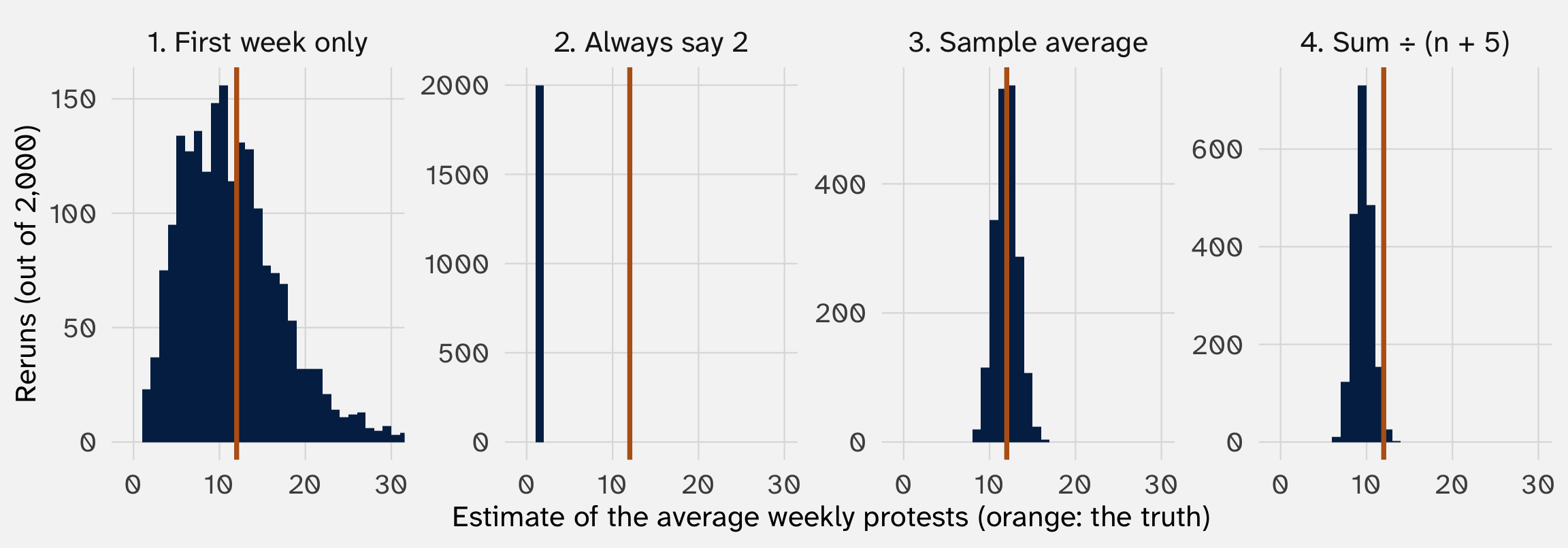
2,000 reruns: each draws a fresh sample of 20 weeks and applies four() to it. Each estimator is a random variable, and its properties are properties of its sampling distribution: where it’s centered, and how spread out it is
Finite-sample properties: unbiased and efficient
Bias: is the sampling distribution centered on the truth?
\[ \text{Bias}(\hat{\mu}) = E[\hat{\mu}] - \mu \]
An estimator is unbiased if its bias is 0: on average, across reruns, it lands on the truth
Bias is not the miss of one estimate. One estimate’s miss has two sources, as in week 2:
\[ \underbrace{\hat{\mu} - \mu}_{\text{one estimate's miss}} \;=\; \underbrace{E[\hat{\mu}] - \mu}_{\text{bias}} \;+\; \underbrace{\hat{\mu} - E[\hat{\mu}]}_{\text{noise}} \]
Bias by hand: three rules from week 5, and one fact about our data
| Rule | In symbols |
|---|---|
| The expectation of a constant is that constant | \(E[c] = c\) |
| Constants come out of an expectation | \(E[kX] = k \, E[X]\) |
| The expectation of a sum is the sum of the expectations | \(E[X + Y] = E[X] + E[Y]\) |
Our data: each \(Y_i\) is one randomly drawn week from the population, so it’s equally likely to be any of the 10,000 (iid)
Its expected value is the population average: \(E[Y_i] = E[Y_1] = E[Y_2] = \dots = \mu\)
Estimators 1 and 2: the centers are immediate
Estimator 1, the first week: \(E[\hat{\mu}_1] = E[Y_1] = \mu\). Unbiased. Surprising?
A single randomly drawn week is sometimes high and sometimes low, but across reruns it’s centered on the truth. Unbiased says nothing about how far one estimate lands from the truth. That’s the spread, and for Estimator 1 it is large (a few slides from now)
Estimator 2, always say 2: \(E[\hat{\mu}_2] = E[2] = 2\), so its bias is \(2 - \mu = 2 - 12 = -10\). Biased, by 10 protests a week, at every sample size
Estimator 3, the sample average: step by step
\[ E[\bar{Y}] = E\left[\frac{Y_1 + \cdots + Y_n}{n}\right] \]
\[ = \frac{1}{n} \, E[Y_1 + \cdots + Y_n] \qquad \text{(constants come out)} \]
\[ = \frac{1}{n} \big( E[Y_1] + \cdots + E[Y_n] \big) \qquad \text{(the expectation of a sum is the sum of the expectations)} \]
\[ = \frac{1}{n} (\mu + \cdots + \mu) = \frac{1}{n} \, n\mu = \mu \qquad \text{(each } E[Y_i] = \mu\text{)} \]
Unbiased. Same answer as estimator 1: both are centered on the truth. What will separate them is the spread
Estimator 4, sum ÷ (n + 5): the same steps, one number different
\[ E[\hat{\mu}_4] = E\left[\frac{Y_1 + \cdots + Y_n}{n + 5}\right] = \frac{1}{n + 5} \big( E[Y_1] + \cdots + E[Y_n] \big) = \frac{n\mu}{n + 5} \]
This estimator is biased. In what direction?:
\[ \text{Bias}(\hat{\mu}_4) = \frac{n\mu}{n + 5} - \mu = -\frac{5\mu}{n + 5} \]
At \(n = 20\): \(-5 \times 12 / 25 = -2.4\), so it’s centered on \(12 - 2.4 = 9.6\)
Notice! The bias shrinks as \(n\) grows: at \(n = 100\) it’s \(-0.57\); at \(n = 3{,}000\), \(-0.02\)
The four centers: by the rules, and by simulation
| Estimator | Its expectation | Bias | Center when \(\mu = 12\), \(n = 20\) |
|---|---|---|---|
| 1. First week | \(\mu\) | 0 | 12 |
| 2. Always say 2 | \(2\) | \(2 - \mu\) | 2 |
| 3. Sample average | \(\mu\) | 0 | 12 |
| 4. Sum ÷ (n + 5) | \(\dfrac{n\mu}{n + 5}\) | \(-\dfrac{5\mu}{n + 5}\) | 9.6 |
# A tibble: 4 × 2
  estimator          average
  <fct>                <dbl>
1 1. First week only   12.0
2 2. Always say 2       2
3 3. Sample average    12.0
4 4. Sum ÷ (n + 5) 9.59This is the center of each estimator; next, the spread
The variance of each estimator comes out of week 5’s rules
Say each week’s count has variance \(\sigma^2\), and weeks are independent
| Estimator | Variance |
|---|---|
| 1. First week | \(\sigma^2\) |
| 2. Always say 2 | \(0\) (a constant doesn’t vary) |
| 3. Sample average | \(\sigma^2 / n\) |
| 4. Sum ÷ (n + 5) | \(n \sigma^2 / (n + 5)^2\) |
1. \(\text{Var}(Y_1) = \sigma^2\)
3. \(\text{Var}(\bar{Y}) = \dfrac{1}{n^2} \text{Var}(Y_1 + \cdots + Y_n) = \dfrac{1}{n^2} (\sigma^2 + \cdots + \sigma^2) = \dfrac{n\sigma^2}{n^2} = \dfrac{\sigma^2}{n}\)
(a constant comes out squared; independent variances add)
4. Same steps, with \(\dfrac{1}{(n + 5)^2}\) out front: \(\dfrac{1}{(n + 5)^2} \cdot n\sigma^2 = \dfrac{n\sigma^2}{(n + 5)^2}\)
Plug in \(\sigma = 6\) and \(n = 20\)
| Estimator | Variance | With the numbers | Spread (SD) |
|---|---|---|---|
| 1. First week | \(\sigma^2\) | \(36\) | \(6\) |
| 2. Always say 2 | \(0\) | \(0\) | \(0\) |
| 3. Sample average | \(\dfrac{\sigma^2}{n}\) | \(\dfrac{36}{20} = 1.8\) | \(\approx 1.34\) |
| 4. Sum ÷ (n + 5) | \(\dfrac{n \sigma^2}{(n + 5)^2}\) | \(\dfrac{20 \times 36}{25^2} \approx 1.15\) | \(\approx 1.07\) |
Number 4 is less variable than number 3: dividing by more than \(n\) shrinks everything, noise included
Lower variance means each estimate lands closer to the estimator’s own center, so all else equal we want it low
But not at any cost! “always say 2” has zero variance, and it’s never right
Efficiency: among unbiased estimators, prefer the smaller variance
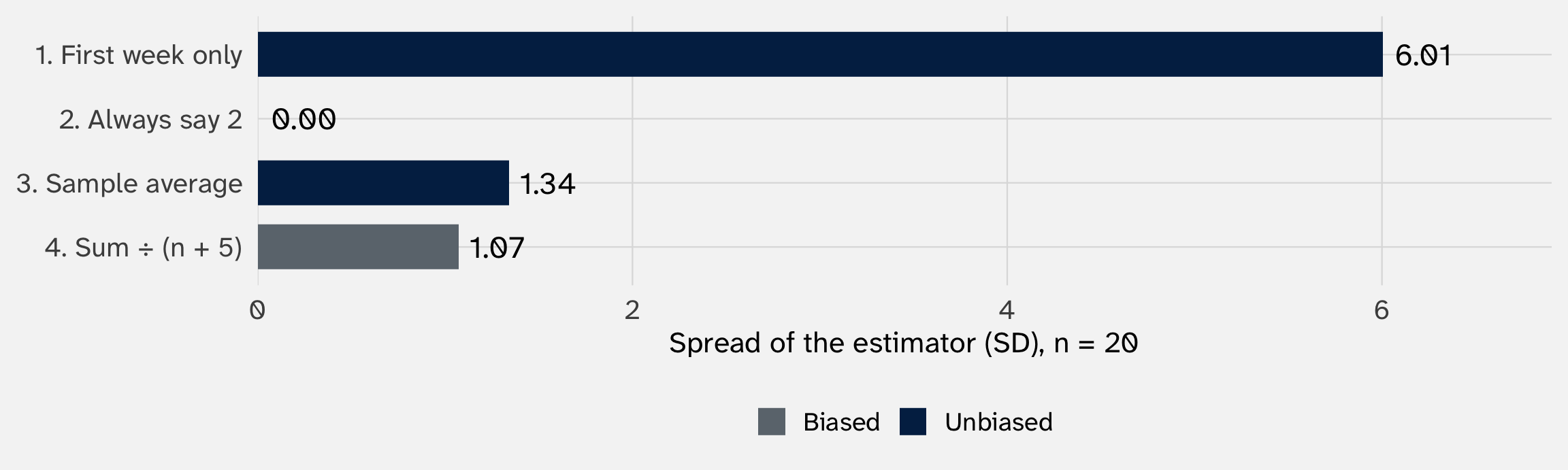
Of the two unbiased estimators, the sample average is more efficient: its variance is \(\sigma^2 / n\), not \(\sigma^2\). It uses all 20 weeks, not one
In other words: if you have two (or more) unbiased estimators, using the less variable one is more efficient (you will be wrong less, in the long run)
Mean squared error
comparing estimators that differ in bias and variance
Bias shifts the cloud of estimates; variance spreads it out
Week 2’s picture, with today’s words. Each blue dot is one rerun’s estimate; the orange dot is the truth
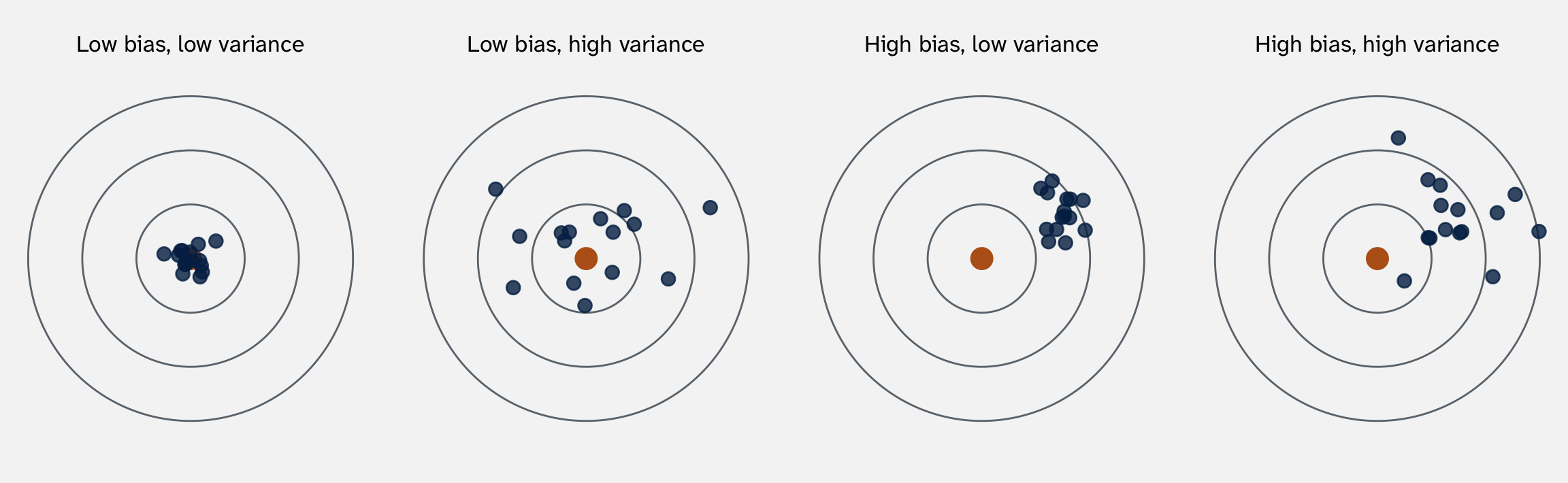
Bias is where the cloud sits; variance is how spread out it is. We want both small
A problem: bias and variance can disagree
| Estimator | Bias | Spread (SD) |
|---|---|---|
| 1. First week | 0.0 | 6.0 |
| 2. Always say 2 | -10.0 | 0.0 |
| 3. Sample average | 0.0 | 1.3 |
| 4. Sum ÷ (n + 5) | -2.4 | 1.1 |
Which is best? Number 4 is biased but tighter than number 3. Number 2 has no spread and a huge bias. Efficiency only compares unbiased estimators, so it can’t rank 3 against 4, or say anything about 2
We need one number that accounts for both: a measure of how far an estimator typically lands from the truth
Mean squared error: the average squared miss, bias and variance together
Week 3: the best guess for a number has the smallest average squared miss. Same idea for an estimator: its average squared miss from the truth, across reruns
\[ \text{MSE}(\hat{\mu}) = E\big[(\hat{\mu} - \mu)^2\big] = \underbrace{\text{Bias}(\hat{\mu})^2}_{\text{how far off-center}} + \underbrace{\text{Var}(\hat{\mu})}_{\text{how scattered}} \]
What it tells us: how far a typical rerun lands from the truth, with both sources of error counted. Its square root is a typical miss in protests. Lower is better, for any estimator, biased or not
And it shows the trade: a biased estimator can still win, if its variance is small enough
A tiny example, by hand
Proof by example that \[ \text{MSE}(\hat{\mu}) = E\big[(\hat{\mu} - \mu)^2\big] = \underbrace{\text{Bias}(\hat{\mu})^2}_{\text{how far off-center}} + \underbrace{\text{Var}(\hat{\mu})}_{\text{how scattered}} \]
An estimator of \(\mu = 12\) lands on 8 half the time and on 12 half the time
| Value | Probability | Miss | Squared miss |
|---|---|---|---|
| 8 | 1/2 | \(-4\) | 16 |
| 12 | 1/2 | 0 | 0 |
\(\text{MSE} = \tfrac{1}{2}(16) + \tfrac{1}{2}(0) = 8\)
Now the pieces. Its center is \(\tfrac{1}{2}(8) + \tfrac{1}{2}(12) = 10\), so the bias is \(10 - 12 = -2\). Its variance is \(\tfrac{1}{2}(8 - 10)^2 + \tfrac{1}{2}(12 - 10)^2 = 4\)
\[ \text{Bias}^2 + \text{Var} = 4 + 4 = 8 \; \checkmark \]
The four estimators: which one misses least?
| Estimator | Bias squared | Variance | MSE | Typical miss, √MSE |
|---|---|---|---|---|
| 1. First week only | 0.00 | 36.06 | 36.06 | 6.0 |
| 2. Always say 2 | 100.00 | 0.00 | 100.00 | 10.0 |
| 3. Sample average | 0.00 | 1.80 | 1.80 | 1.3 |
| 4. Sum ÷ (n + 5) | 5.76 | 1.15 | 6.91 | 2.6 |
The sample average wins: a typical miss of 1.3 protests a week. The adjusted average is biased, but its low variance keeps it close (2.6). The first week alone misses by 6; “always say 2” by 10
Which estimator wins depends on the truth, and we don’t know the truth
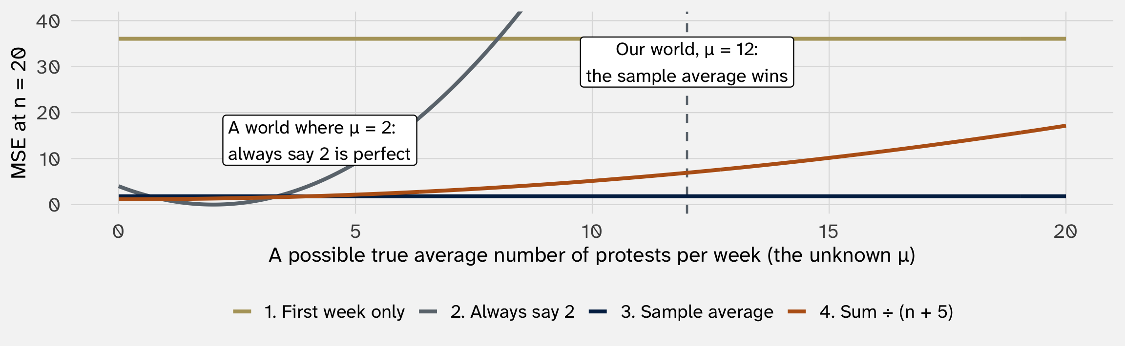
How to read it: each point on the x-axis is a possible world, with a different true average. A line’s height there is how badly its estimator does (lower is better)
“Always say 2” is perfect if the truth is 2, and terrible elsewhere. In our world (dashed), the sample average is lowest, and its line is flat: it does well whatever \(\mu\) is. We never know which world we’re in
Asymptotic properties: consistent
More data: do the estimators close in on the truth?
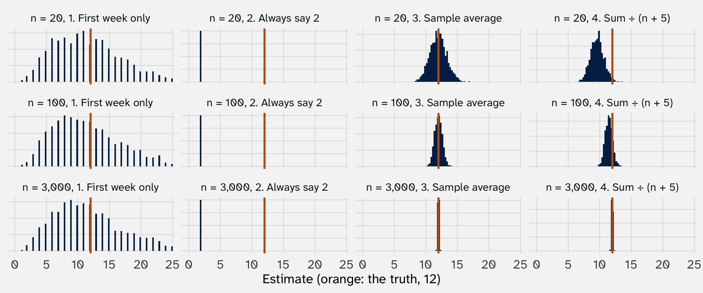
The first week and “always say 2” never improve. The other two close in on 12, though the adjusted one is biased at every \(n\)
Consistency: the estimator closes in on the truth as \(n\) grows
An estimator is consistent if, for any small distance \(\varepsilon\), the chance it misses the truth by \(\varepsilon\) or more goes to zero as \(n\) grows:
\[ P(|\hat{\mu}_n - \mu| \geq \varepsilon) \rightarrow 0 \quad \text{as } n \rightarrow \infty \]
| Estimator | Unbiased? | Consistent? | Why |
|---|---|---|---|
| 1. First week | Yes | No | Still one week of data, however big the sample |
| 2. Always say 2 | No | No | Ignores the data |
| 3. Sample average | Yes | Yes | The law of large numbers (week 6) |
| 4. Sum ÷ (n + 5) | No | Yes | Its bias, \(-5\mu / (n + 5)\), and its variance both shrink to 0 |
Unbiased and consistent are different ideas. One is about the center at a given \(n\); the other is about what happens as \(n\) grows. Neither implies the other
The sample average has all four properties
| Estimator | Unbiased (finite-sample) | Efficient (finite-sample) | Consistent (asymptotic) | Asymp. normal (asymptotic) |
|---|---|---|---|---|
| 1. First week | Yes | No | No | No |
| 2. Always say 2 | No | n/a | No | n/a |
| 3. Sample average | Yes | Yes | Yes | Yes |
| 4. Sum ÷ (n + 5) | No | n/a | Yes | Yes |
Asymptotically normal: by the CLT, for large \(n\) the sample average’s sampling distribution is about \(N(\mu, \sigma^2 / n)\). That’s the bell behind “95% of studies land within 2 standard errors”
Number 4 gets a bell too: it’s a rescaled average, \(\hat{\mu}_4 = \frac{n}{n + 5} \, \bar{Y}\), and \(\frac{n}{n + 5} \rightarrow 1\)
So we’ve proved the seemingly obvious: for an average, the sample average is a good estimator. But when is the obvious estimator less obvious?
When the obvious estimator is less obvious
Counting the dead: the estimand is a total, not an average
We want \(N\), the total number of people killed in a conflict. It’s not an average of anything we observe
Two groups have been collecting names: a truth commission and a human-rights NGO. Each list is incomplete: some killings were never reported to either one
The “obvious” estimator: count the names we have. Is that a good estimator of \(N\)? Which way will it be biased?
It can never exceed \(N\), so its sampling distribution can’t be centered on \(N\). It’s biased low, by construction
How low? We can’t count the dead nobody recorded. But the two lists carry information about each other: how much do they overlap?
This is called capture–recapture in ecology (tag animals, release them, catch again, and see what share are tagged), and multiple systems estimation in conflict research, where the “catches” are lists of the dead
Two lists tell us how much each one misses
Suppose the commission’s list has 600 names, the NGO’s has 400, and 200 names are on both
The NGO caught 200 of the commission’s 600: one in three. The commission’s names are a sample of the dead, so the NGO’s catch rate among them is our estimate of its catch rate among everyone: one in three
If the NGO catches a third of everyone, its 400 names are a third of the total:
\[ \hat{N} = \frac{400}{1/3} = 1{,}200 \qquad \text{or, in general,} \qquad \hat{N} = \frac{n_A \times n_B}{\text{names on both}} = \frac{600 \times 400}{200} \]
Why is that leap sensible? It works if the NGO is equally likely to record a death whether or not the commission did. Then the commission’s names are, as far as the NGO is concerned, a random look at the dead. If the commission’s names are special (say, the easy-to-document deaths), the NGO’s catch rate among them tells us little about its catch rate overall
Check it in a world where we know the truth
As all term, we write the world, so we can judge the estimators. 1,200 people were killed. The commission records each death with chance \(1/2\), the NGO with chance \(1/3\), and independently
Expected names: commission \(1{,}200 \times \tfrac{1}{2} = 600\); NGO \(1{,}200 \times \tfrac{1}{3} = 400\); both \(1{,}200 \times \tfrac{1}{2} \times \tfrac{1}{3} = 200\) (independent chances multiply). So names on either list: \(600 + 400 - 200 = 800\)
| Estimator | Average across 2,000 simulated reruns | Bias (average minus 1,200) |
|---|---|---|
| Names we have (on either list) | 800 | -400 |
| Two lists: \(n_A \times n_B\) ÷ overlap | 1,202 | 2 |
The names we have are 400 short, a third of the truth. The two-list estimate is centered on the truth (we know because we know \(N\))
A real case: how many died in Peru’s civil war?
Peru’s truth commission matched several lists and found 24,692 documented deaths. Using the lists method, Ball et al. estimated about 69,280 (Ball et al. 2003)
Then the number moved. A reanalysis argued the method distorted the total: about 48,000 (Rendón 2019). A later one, with more data: about 58,000 (Manrique-Vallier, Ball, and Sulmont 2019). Same lists, different assumptions about how they were generated, different answers
The lists method is now widely used: truth commissions and courts have relied on it to estimate the dead in Guatemala, Kosovo, Timor-Leste, and Colombia
References
Ball, Patrick, Jana Asher, David Sulmont, and Daniel Manrique. 2003. How Many Peruvians Have Died? An Estimate of the Total Number of Victims Killed or Disappeared in the Armed Internal Conflict Between 1980 and 2000. American Association for the Advancement of Science. Report.
Manrique-Vallier, Daniel, Patrick Ball, and David Sulmont. 2019. “Estimating the Number of Fatal Victims of the Peruvian Internal Armed Conflict, 1980–2000: An Application of Modern Multi-List Capture-Recapture Techniques.”
Rendón, Silvio. 2019. “Capturing Correctly: A Reanalysis of the Indirect Capture–Recapture Methods in the Peruvian Truth and Reconciliation Commission.” Research & Politics 6(1). doi:10.1177/2053168018820375.
Xu, Yiqing. 2026. “Point Estimation.” https://github.com/xuyiqing/regression-lectures.
POL 211 · Fall 2026