POL 211 · Week 6
University of California, Davis
November 3, 2026

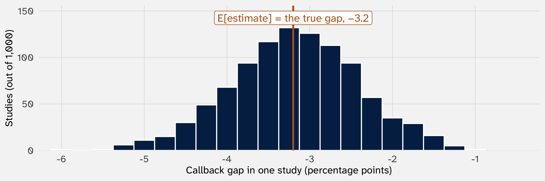
\(E[\hat{\Delta}] = \Delta\): the difference in callback rates is unbiased for the gap. Randomizing the names is what makes that gap the effect of the name
\[ \text{SD}(\hat{\Delta}) = \sqrt{ \frac{\overbrace{p_{\text{AA}}(1 - p_{\text{AA}})}^{\text{a coin flip's variance}}}{\underbrace{n_{\text{AA}}}_{\text{averaging independent flips}}} \overbrace{+}^{\text{independent groups}} \frac{p_{\text{white}}(1 - p_{\text{white}})}{n_{\text{white}}} } \]
The classic standard error assumes independence. Without it, the variance of a sum picks up a covariance term for every pair of résumés, and this SE is too narrow (more at the end of today)
We never see \(p_{\text{AA}}\) or \(p_{\text{white}}\). So we plug in the callback shares from the one run of data we have:
\[ \widehat{SE}(\hat{\Delta}) = \sqrt{\frac{\hat{p}_{\text{AA}}(1 - \hat{p}_{\text{AA}})}{n_{\text{AA}}} + \frac{\hat{p}_{\text{white}}(1 - \hat{p}_{\text{white}})}{n_{\text{white}}}} = \sqrt{\frac{0.064(1 - 0.064)}{2{,}435} + \frac{0.097(1 - 0.097)}{2{,}435}} = 0.0078 \]
So the standard error in week 1’s table is itself an estimate: a guess, from one run of data, at the width of a distribution we can’t see (Wooldridge 2023, 2)
Is that OK? \(\hat{p}\) isn’t \(p\). Today’s first question: why would plugging in \(\hat{p}\) work?

But no single résumé’s outcome looks like a bell. A callback is a 0 or a 1
Today’s second question: why does the sampling distribution look like a bell?
| Question | Answer |
|---|---|
| Where does the sampling distribution sit? | On the truth (week 5) |
| How wide is it? | \(\sigma / \sqrt{n}\), if the draws are independent (week 5) |
| Why can we plug in \(\hat{p}\) for \(p\)? | Averages settle on their expectation: the law of large numbers |
| How do we describe a bell? | The normal distribution (which needs continuous random variables first) |
| Why is the sampling distribution a bell? | The central limit theorem |
| What does the bell buy us? | About 95% of studies land within 2 standard errors of the truth |
Last week’s standard error leaned on independence: it wiped out the covariance term for every pair of résumés. Statistics usually states that assumption as iid:
The résumé study isn’t identically distributed: each résumé has its own \(p_i\). That’s fine. Week 5 showed the share still centers on the average \(p_i\), and today’s results allow it too, as long as no handful of draws dominates the average
Independence is the more common violation. The end of today shows what happens without it
Take iid draws \(X_1, X_2, \ldots, X_n\), each with mean \(\mu\). As \(n\) grows, their average gets closer and closer to \(\mu\):
\[ \bar{X}_n \rightarrow \mu \quad \text{as } n \rightarrow \infty \]
For coin flips, \(\mu = p\) and the average is the share of 1s, so \(\hat{p} \rightarrow p\)
This holds for any distribution with a mean: a die, a thermometer score, a protest’s size
The precise version says the chance \(\bar{X}_n\) lands more than any tiny distance from \(\mu\) shrinks to zero (“convergence in probability”). Week 7 calls an estimator that does this consistent

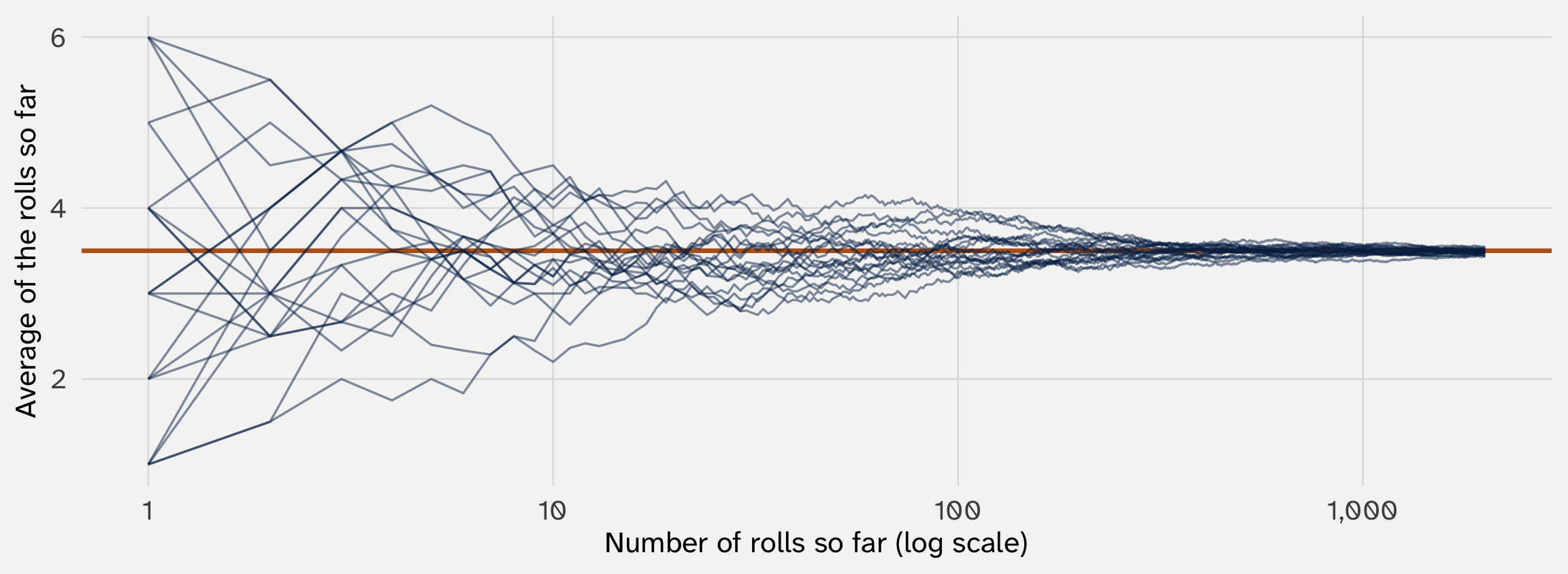
Each line is one person rolling 2,000 times. After every roll, they compute the average of all their rolls so far. Orange: the expectation of one roll, \(E[X] = 3.5\)

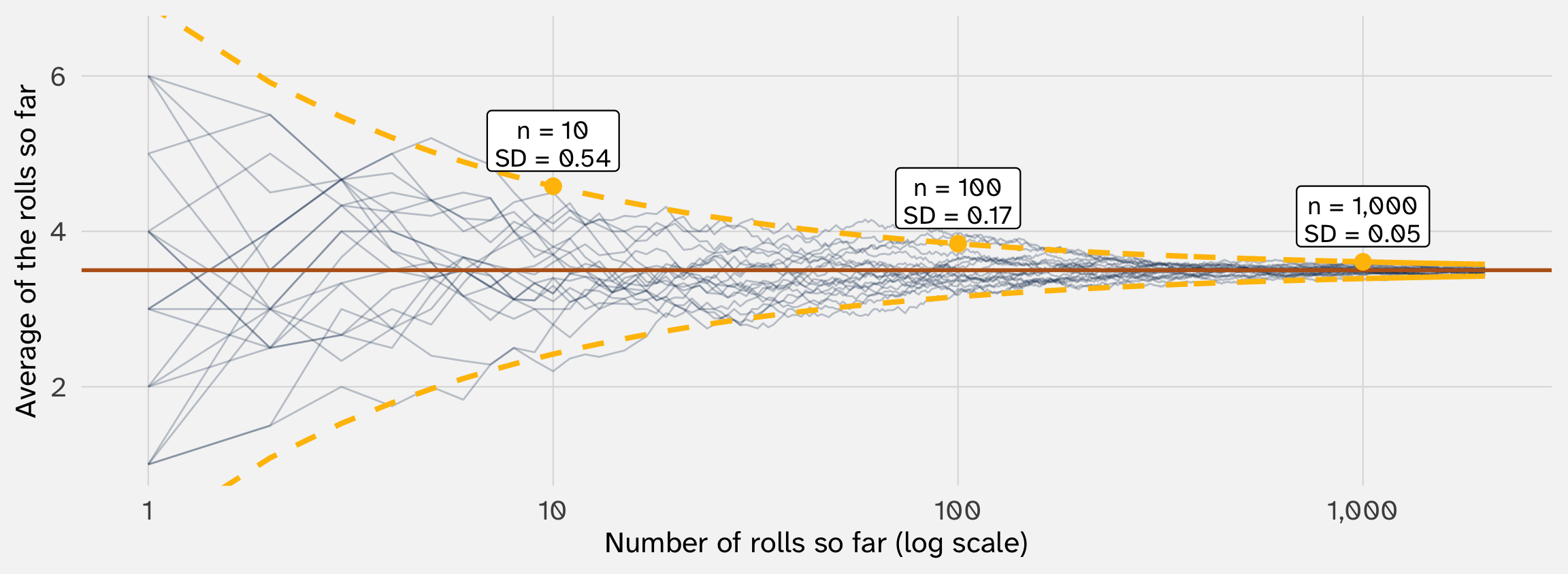
Gold: \(3.5 \pm 2\sigma/\sqrt{n}\), with \(\sigma =\) 1.71 for one roll. Ten times the rolls, a third of the width. Week 5’s formula is the LLN’s speed
Picture a classroom. You know two things: average height and the standard deviation (SD = 3). That means their variance (the average squared distance from the mean) is 9
Chebyshev says that if you know the spread, only so many kids can be really far from the average. The reason is that variance works like a budget. Each kid “spends” from it according to the square of their distance from the average. A kid \(3\delta\) away costs 9 units, so a lot of kids that far out would “use up” more spread than the class has
Formally, for any distribution at all:
\[ P(|X - \mu| \geq k\sigma) \leq \frac{1}{k^2} \]
| Distance from the mean | Chebyshev’s cap, any distribution | A normal distribution |
|---|---|---|
| 2 or more SDs | 1/4 = 25% | 4.6% |
| 3 or more SDs | 1/9 = 11% | 0.3% |
| 10 or more SDs | 1/100 = 1% | about 0% |
It assumes nothing about the shape, only a finite variance
Averaging cancels noise, so the spread of the average shrinks: \(\text{Var}(\bar{X}) = \sigma^2 / n\) (the funnel)
Chebyshev, applied to \(\bar{X}\), bounds the chance it misses the truth by \(\varepsilon\) or more:
\[ P(|\bar{X}_n - \mu| \geq \varepsilon) \leq \frac{\sigma^2}{n \, \varepsilon^2} \]
Hold \(\varepsilon\) fixed, however tiny, and let \(n\) grow: the right side goes to 0. That’s the law of large numbers
A die: \(\sigma^2 = 2.92\) (Problem Set 5). Take \(\varepsilon = 0.1\), so \(\varepsilon^2 = 0.01\):
\[ n = 1{,}000: \;\; \frac{2.92}{1{,}000 \times 0.01} = \frac{2.92}{10} \approx 0.29 \qquad\qquad n = 10{,}000: \;\; \frac{2.92}{10{,}000 \times 0.01} = \frac{2.92}{100} \approx 0.03 \]
At most 29% of averages of 1,000 rolls miss 3.5 by 0.1 or more; at most 3% of averages of 10,000
A small spread means the average can’t wander far. More data shrinks the spread toward zero. So with enough data, the average can’t wander far from the truth
\(\hat{p}_{\text{AA}}\) is the average of 2,435 coin flips, each with expectation \(p_{\text{AA}}\). So the LLN says \(\hat{p}_{\text{AA}} \rightarrow p_{\text{AA}}\)
And if \(\hat{p}\) lands close to \(p\), then \(\hat{p}(1 - \hat{p})\) lands close to \(p(1 - p)\). So the plug-in standard error lands close to the true width:
\[ \widehat{SE}(\hat{\Delta}) \rightarrow \text{SD}(\hat{\Delta}) \quad \text{as } n \rightarrow \infty \]
With a few thousand résumés, the plug-in barely matters. With a few dozen, it can

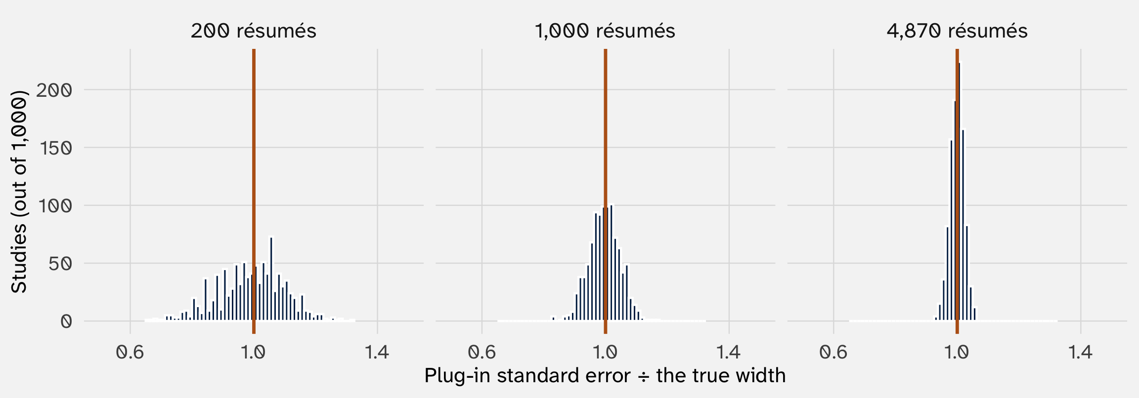
Each study plugs its own \(\hat{p}\)’s into the formula; the true width plugs in the true \(p\)’s, which we know because we wrote the DGP. With 200 résumés, 65% of studies land within 10% of the truth. With 4,870, 100% do

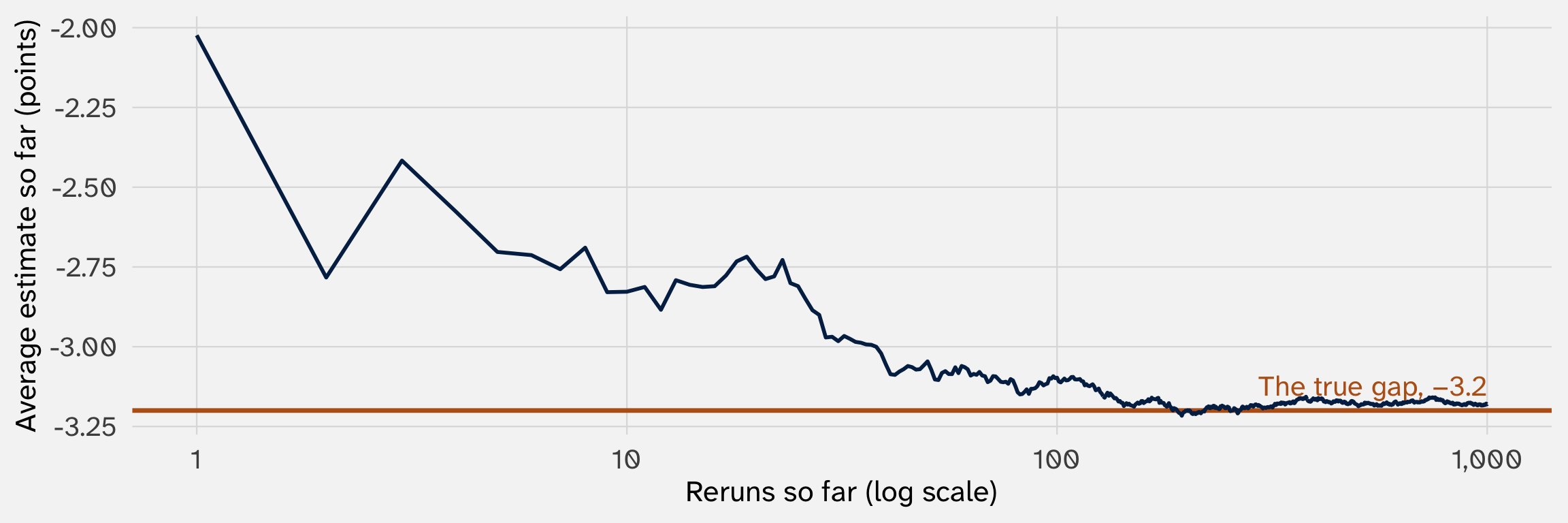
Week 4’s 1,000 reruns of the résumé study: the average of the estimates so far settles on the truth. Every “check it by simulation” slide leaned on this
set.seed(211)
canvass = tibble(dem = rbinom(1000, size = 1, prob = 0.5), # a coin flip: Democrat or not
canvassed = rbinom(1000, size = 1, prob = 0.5)) |> # a coin flip: canvassed or not
mutate(systematic = 40 + # an uncanvassed non-Democrat
5 * canvassed + # a knock on the door: +5 points (the effect)
20 * dem) # a registered Democrat: +20 points
canvass# A tibble: 1,000 × 3
dem canvassed systematic
<int> <int> <dbl>
1 0 0 40
2 1 1 65
3 1 0 60
4 0 1 45
5 0 0 40
# ℹ 995 more rows
The average score for voters with these inputs. It takes just four values: 40, 45, 60, or 65
# A tibble: 1,000 × 5
dem canvassed systematic noise therm
<int> <int> <dbl> <dbl> <dbl>
1 0 0 40 27.1 67.1
2 1 1 65 -12.6 52.4
3 1 0 60 17.1 77.1
4 0 1 45 8.90 53.9
5 0 0 40 13.6 53.6
# ℹ 995 more rows
rnorm() draws each voter’s noise. A real researcher sees dem, canvassed, and therm, not the two parts
# A tibble: 2 × 2
canvassed average_therm
<int> <dbl>
1 0 50.1
2 1 53.8
The difference in means: 3.8 points. The true effect we built in: 5
With the résumés we only ever talked about \(p\). For a coin flip, \(p\) pins down everything: the whole distribution (\(P(Y = 1) = p\)), the center (\(p\)), and the spread (\(p(1 - p)\)). The random part came along for free
The canvass is different. The systematic part (40, 45, 60, or 65) gives the center but says nothing about the spread. The spread lives in the noise
And we need that spread: the random part is what makes estimates vary from study to study (week 4), so its variance is what goes into the standard error.
The noise can be any number: 3.7, −12.04, 26.519… So unlike a Bernoulli, it is a continuous random variable
| Discrete: a list of separate values | Continuous: any value in a range | |
|---|---|---|
| Examples | A callback (0/1), votes cast, protests in a year | A thermometer score, income, a vote share, days until a ceasefire breaks |
| The distribution | A probability for each value | A density: a curve |
| Probability of a single value | Can be big: \(P(Y = 1) = 0.08\) | Zero |
| Probability of a range | Add up the bars | Area under the curve |

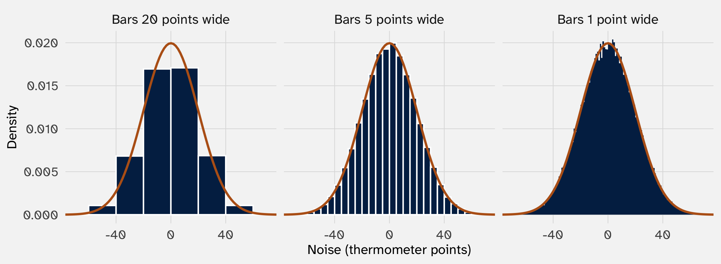
The orange curve is the density, \(f(x)\): what the histogram becomes with infinitely many draws and infinitely thin bars

# A tibble: 1 × 1
exactly_3.7
<int>
1 0
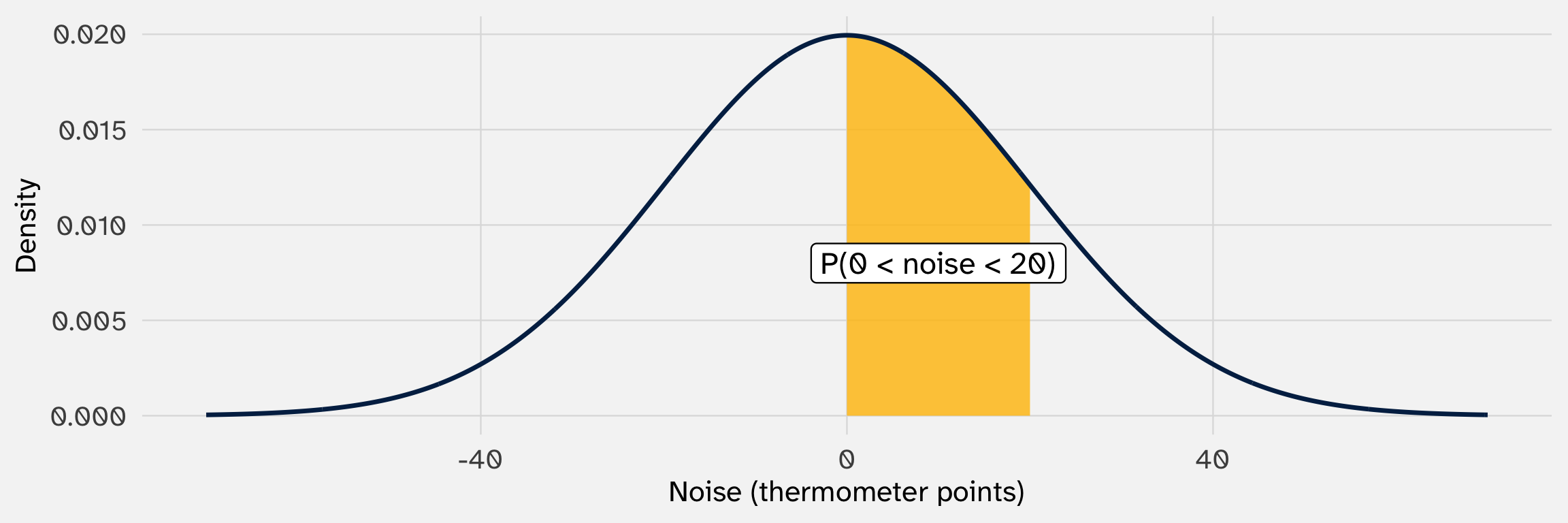
A single point has no width, so it has no area: \(P(\text{noise} = 3.7) = 0\)
So with continuous variables we always ask about ranges: \(P(3.65 < X < 3.75)\), \(P(X > 20)\)
| Discrete | Continuous | |
|---|---|---|
| Expectation | \(E[X] = \sum_x x \cdot P(X = x)\) | \(E[X] = \int x \cdot f(x) \, dx\) |
| Variance | \(\text{Var}(X) = \sum_x (x - E[X])^2 \, P(X = x)\) | \(\text{Var}(X) = \int (x - E[X])^2 f(x) \, dx\) |
\(\int\) is a sum over infinitely many, infinitely thin slices. Same idea: each value, weighted by how likely it is
And every rule from week 5 still holds: \(E[X + Y] = E[X] + E[Y]\), \(\text{Var}(kX) = k^2 \text{Var}(X)\), the sum rule with its covariance term, \(\sigma^2 / n\)

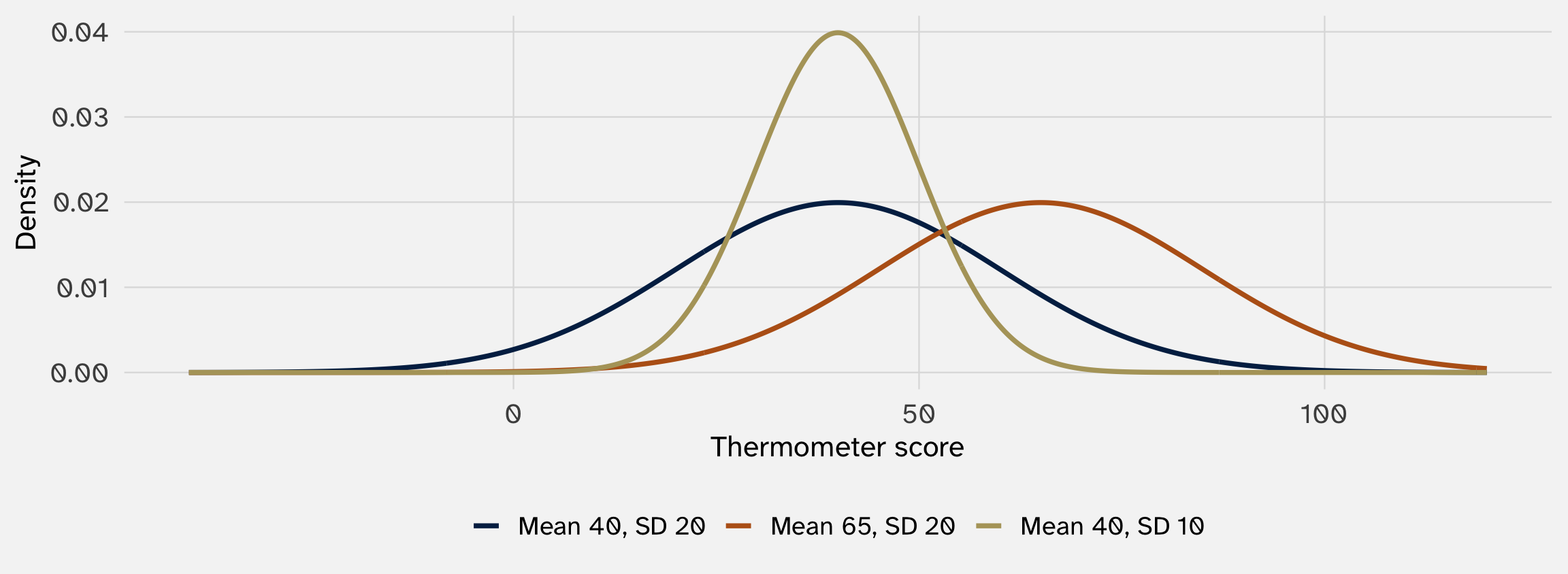
\(X \sim N(\mu, \sigma^2)\): the mean \(\mu\) moves the bell, the SD \(\sigma\) stretches it. Symmetric, with thin tails
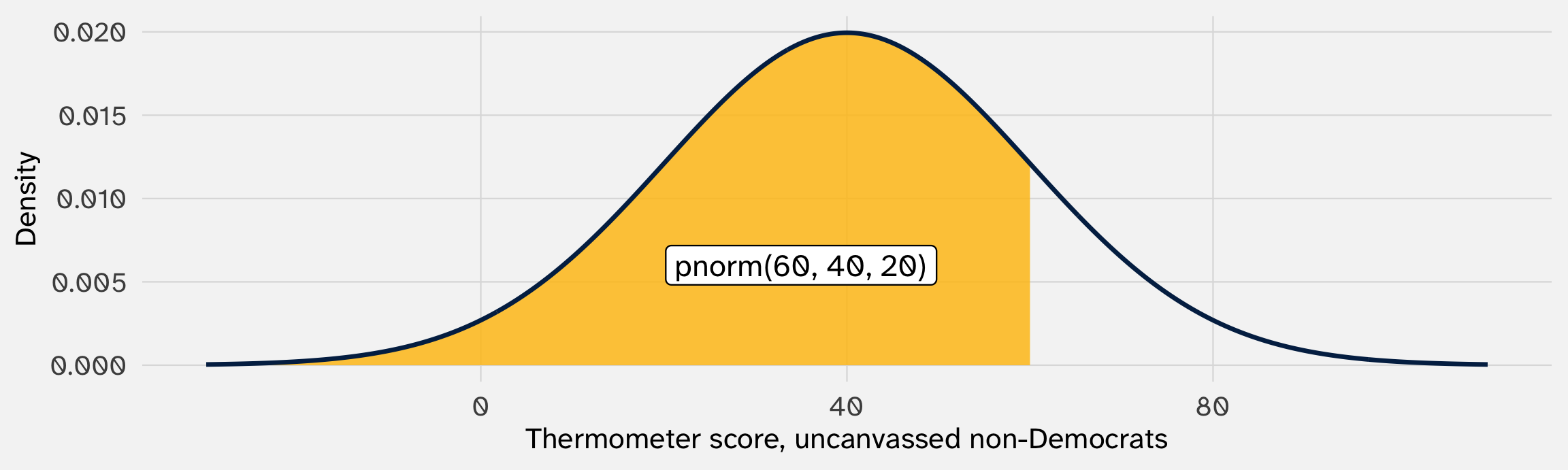
The noise is \(N(0, 20^2)\). Fix a voter’s inputs and the systematic part is just a number. For a non-Democrat nobody canvassed:
\[ \texttt{therm} = \underbrace{40 + 5(0) + 20(0)}_{= \, 40} + \text{noise} \;\sim\; N(40, 20^2) \]
| One unit’s outcome | Its inputs | Systematic part | Its distribution |
|---|---|---|---|
| Résumé #1’s callback, \(Y_1\) | Its name, experience, age, distance | \(p_1 = 0.0545\) | \(\text{Bernoulli}(0.0545)\) |
| A voter’s thermometer score | Not canvassed, not a Democrat | \(40 + 0 + 0 = 40\) | \(N(40, 20^2)\) |
| Not canvassed, a Democrat | \(40 + 0 + 20 = 60\) | \(N(60, 20^2)\) | |
| Canvassed, not a Democrat | \(40 + 5 + 0 = 45\) | \(N(45, 20^2)\) | |
| Canvassed, a Democrat | \(40 + 5 + 20 = 65\) | \(N(65, 20^2)\) |
Each unit’s outcome is a random variable, and its systematic part sets the center. For a coin flip, the center also fixes the spread, \(p(1 - p)\). The canvass noise has its own spread: SD 20 for every voter

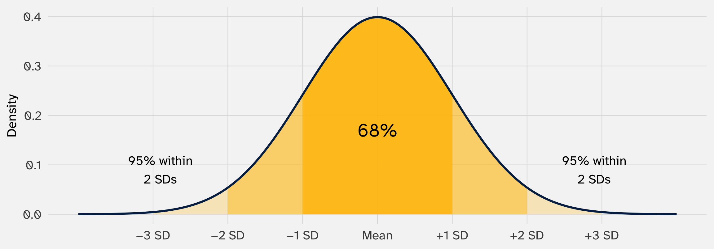
For any normal: 68% of draws within one SD of the mean, 95% within two, 99.7% within three
Take any \(X\) with mean \(\mu\) and SD \(\sigma\), and standardize it:
\[ Z = \frac{X - \mu}{\sigma} \]
\[ E[Z] = \frac{E[X] - \mu}{\sigma} = 0 \qquad \text{Var}(Z) = \frac{\text{Var}(X)}{\sigma^2} = \frac{\sigma^2}{\sigma^2} = 1 \]
The shift rule moves the center to 0; the \(k^2\) rule (with \(k = 1/\sigma\)) shrinks the variance to 1
If \(X\) is normal, \(Z \sim N(0, 1)\). \(Z\) counts SDs from the mean: the z-score
An uncanvassed non-Democrat: \(\texttt{therm} = 40 + \text{noise} \sim N(40, 20^2)\). One of them scores 80
\[ z = \frac{80 - 40}{20} = 2 \]
Two SDs above the mean: warmer than about 97.7% of voters like them. A canvassed Democrat who scores 80 has \(z = (80 - 65)/20 = 0.75\): warmer than about 77%
| Function | What it gives | Normal | You’ve used |
|---|---|---|---|
r*() |
Random draws | rnorm(n, mean, sd) |
rnorm(), rbinom() since Problem Set 1 |
d*() |
The density’s height (a probability, for discrete) | dnorm(x, mean, sd) |
the curves on these slides |
p*() |
The area to the left of \(x\): \(P(X \leq x)\) | pnorm(x, mean, sd) |
new |
q*() |
The \(x\) with a given area to its left | qnorm(p, mean, sd) |
new |
Swap the letters after the first one for other distributions: rbinom(), dbinom(), pbinom(), qbinom()
pnorm() gives the area to the left
qnorm() runs pnorm() backwardWhich score marks the top 2.5%? Ask for the point with 97.5% of the area to its left:
[1] 79.19928
[1] 1.959964
1.96: the middle 95% of any normal runs from 1.96 SDs below the mean to 1.96 above. “About 2” in the 68–95–99.7 rule is 1.96. You will see this number for the rest of your career
pnorm() and qnorm()In the canvass DGP:
Check one of your answers with rnorm() draws
pnorm() and qnorm(): answers| The average of \(n\) independent draws, \(\bar{X}\) | Where it comes from | |
|---|---|---|
| Center | \(E[\bar{X}] = \mu\) | Week 5: the expectation of a sum |
| Width | \(\text{SD}(\bar{X}) = \sigma / \sqrt{n}\) | Week 5: the variance of a sum of independent draws |
| Shape | About normal, when \(n\) is large | Today: the central limit theorem |

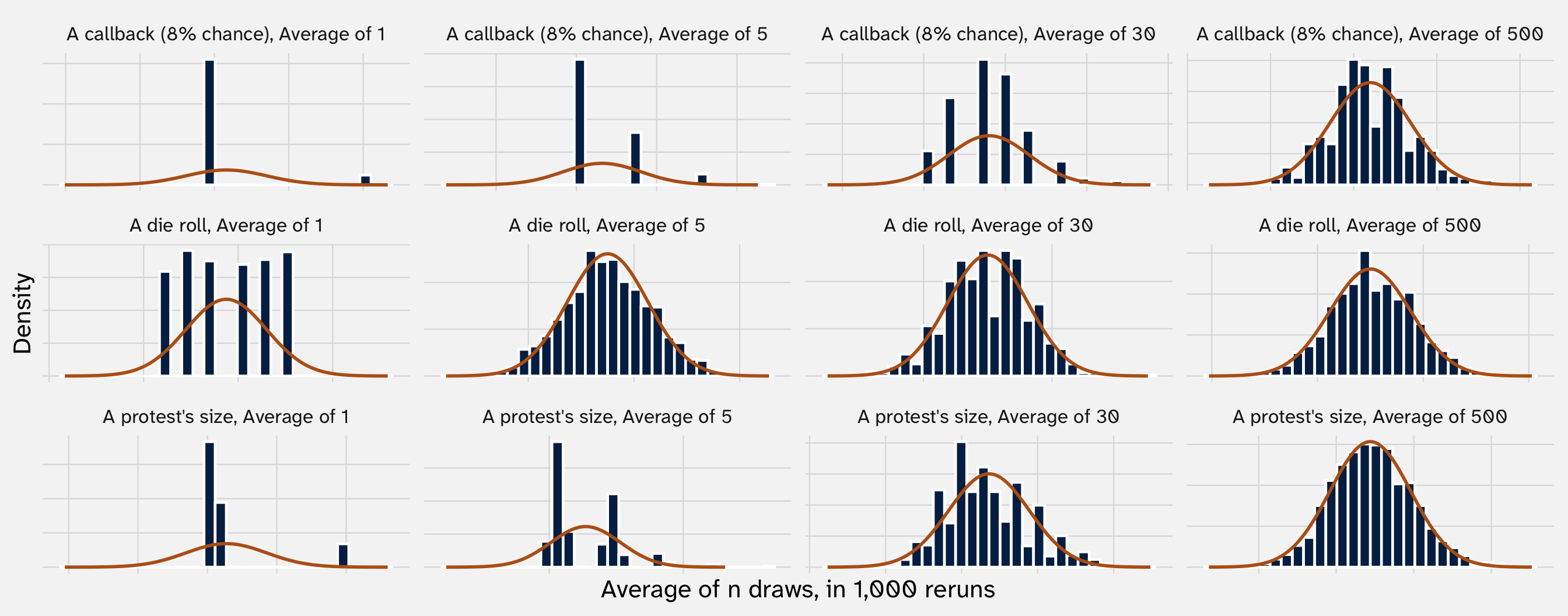
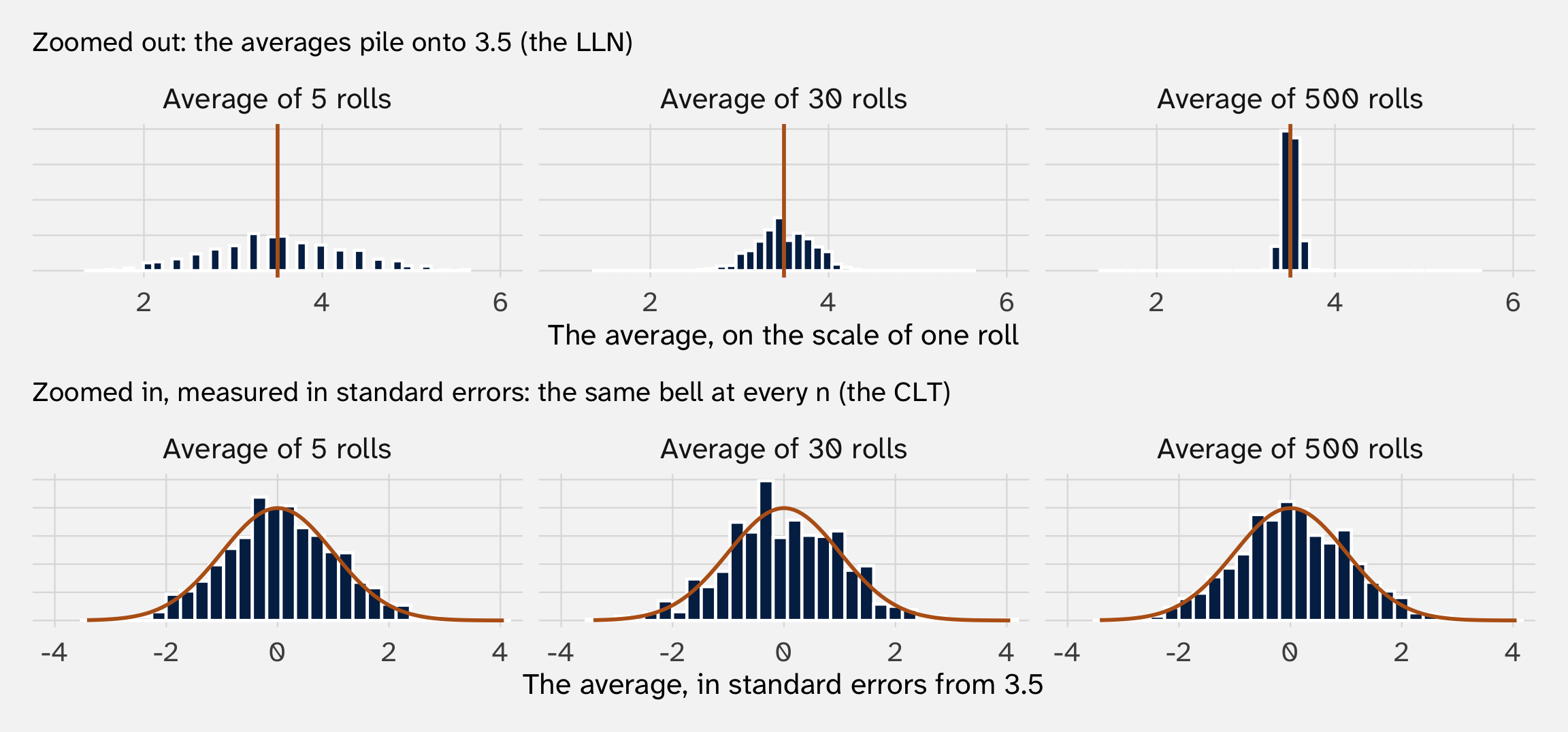
First column, one draw of each: a callback (two bars), a die (flat), a protest’s size (a long right tail). Orange: the normal curve with week 5’s center \(\mu\) and width \(\sigma / \sqrt{n}\)
Take iid draws \(X_1, \ldots, X_n\), each with mean \(\mu\) and variance \(\sigma^2\). When \(n\) is large,
\[ \bar{X} \;\overset{\text{approx.}}{\sim}\; N\!\left(\mu, \; \frac{\sigma^2}{n}\right) \]
Whatever the distribution of one draw. Equivalently, the standardized average is about standard normal:
\[ \frac{\bar{X} - \mu}{\sigma / \sqrt{n}} \;\overset{\text{approx.}}{\sim}\; N(0, 1) \]
“Large” depends on the start: a few draws for a die, hundreds for a rare event or a skewed one

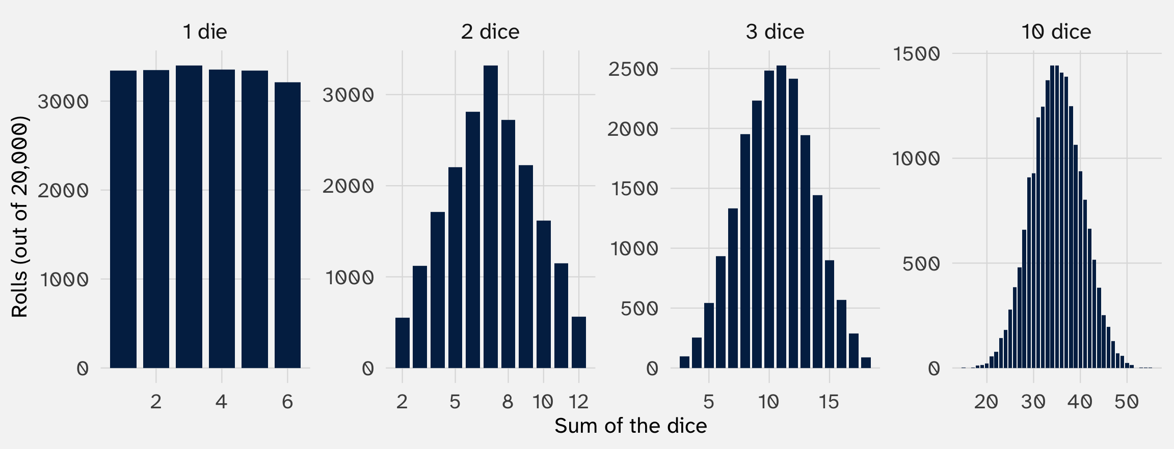
Two dice sum to 12 one way (6 + 6) and to 7 six ways. With ten dice, a sum of 60 needs all ten to show 6; middling sums can happen millions of ways
| Law of large numbers | Central limit theorem | |
|---|---|---|
| The question | Where does the average end up? | What shape is its scatter around that spot? |
| The answer | On the expectation: \(\bar{X} \rightarrow \mu\) | A bell: \(\bar{X} \overset{\text{approx.}}{\sim} N(\mu, \sigma^2 / n)\) |
| As \(n\) grows | The scatter shrinks toward zero | The scatter stays a bell, just narrower |
| What it buys us | \(\hat{p} \rightarrow p\), so the plug-in works; simulations work | About 95% of studies land within 1.96 SEs: confidence intervals and tests (weeks 8 and 9) |
| Today’s picture | The funnel of running averages | The bells in the grid |
One way to keep them straight: the LLN is about one number homing in. The CLT is about the whole distribution of that number on its way there


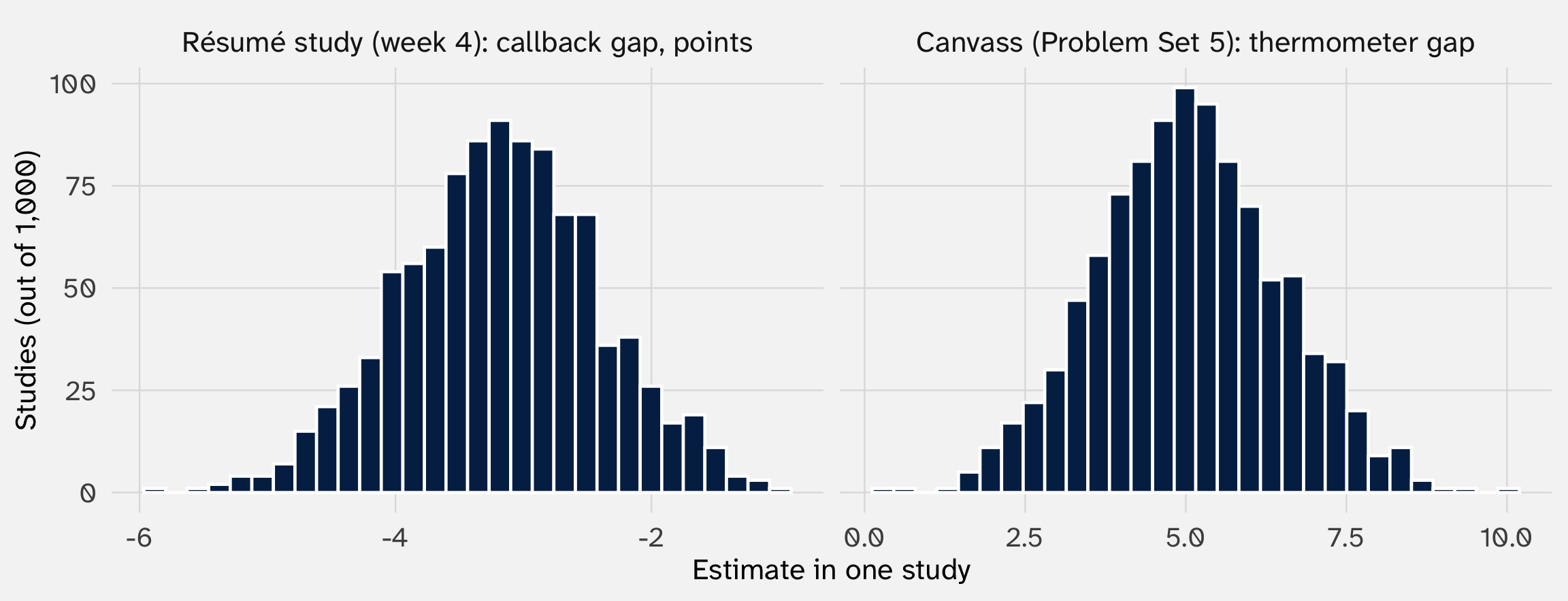
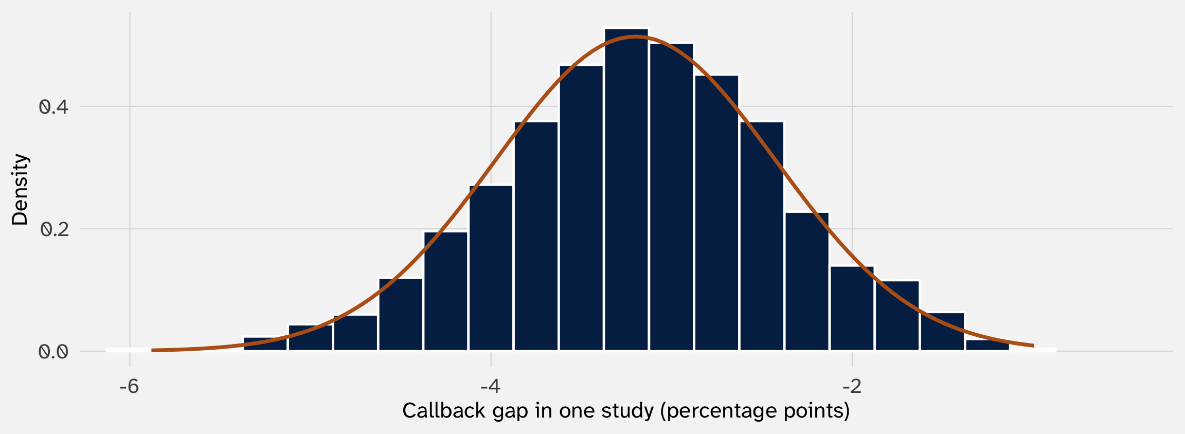
Week 4’s 1,000 reruns, with the normal curve centered at −3.2 points with SD 0.78 points. Each callback share is an average of thousands of coin flips; their difference is normal too
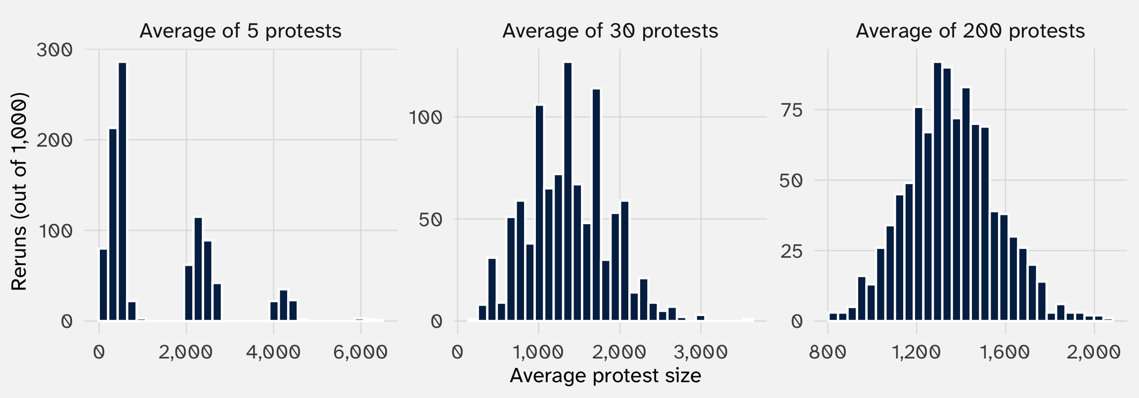
Week 5’s protest: 100 people (probability 0.6), 1,000 (0.3), or 10,000 (0.1)
Mean 1,360, SD about 2,908

Five protests: still skewed. Thirty: close. Two hundred: a bell, with SD 203 against \(2{,}908 / \sqrt{200} \approx\) 206
What if résumés covary? Résumés at one employer share its mood (a 2% chance if the job is filled, 14% if it’s urgent). Orange: the bell week 5’s formula predicts
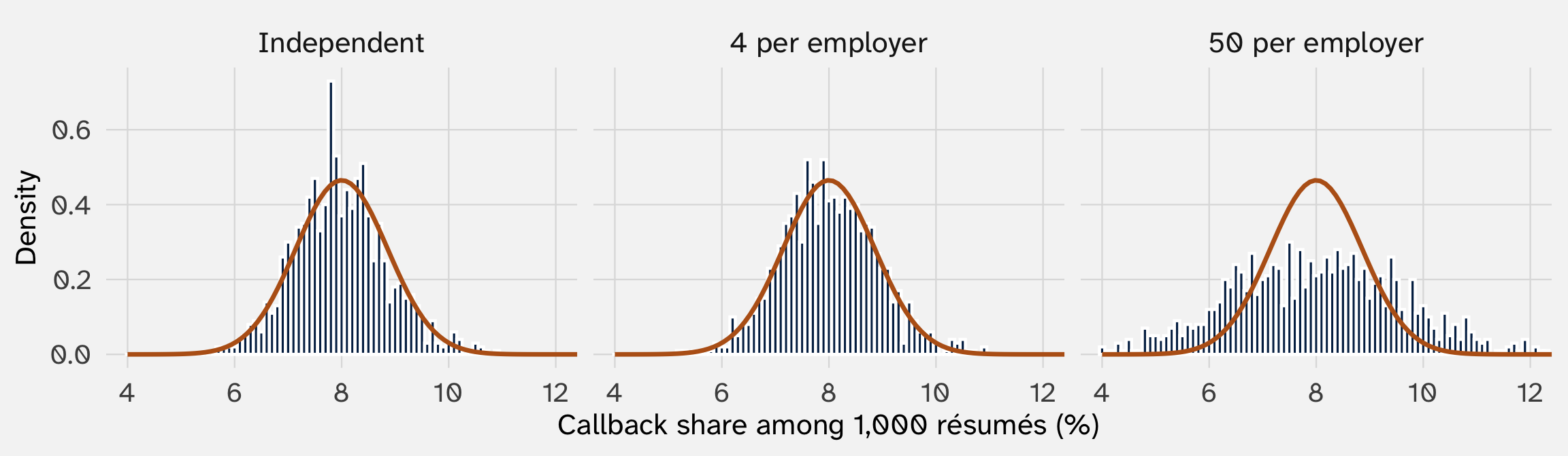
Orange: the bell week 5’s formula predicts
The more résumés share an employer, the wider the real spread. And one decision for all 1,000 (week 5’s scenario B)? The share is 0% or 100%. No bell at all
| Design | Real SD of the share (points) | Formula’s SD (points) | Real ÷ formula | Worth this many independent résumés |
|---|---|---|---|---|
| Independent | 0.85 | 0.86 | 0.99 | 1,015 |
| 4 per employer | 0.89 | 0.86 | 1.04 | 930 |
| 50 per employer | 1.59 | 0.86 | 1.86 | 289 |
| One decision for all | 27.60 | 0.86 | 32.17 | 1 |
Week 5: the variance of a sum has a covariance term for every pair. Independence wipes them all out, which is where \(\sigma^2 / n\) comes from. Linked draws bring them back, so the real spread is bigger than the formula says
Bertrand and Mullainathan sent four résumés to each ad. For the callback share, their 4,870 résumés act like somewhat fewer. Week 10: when to cluster

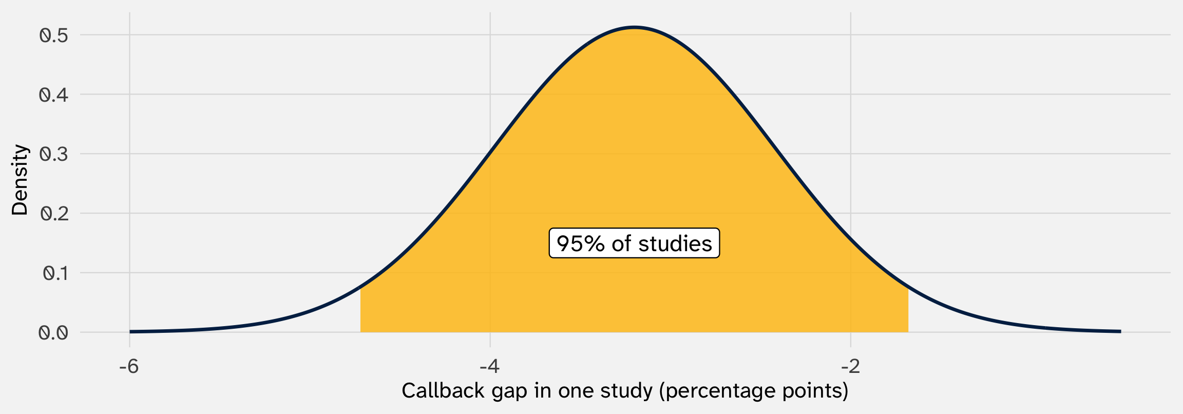
Centered on the truth (week 5), with a standard error of 0.78 points from one run of data (week 5), and normal (today). So 95% of studies land within 1.96 standard errors of the truth
# A tibble: 1 × 1
share_within
<dbl>
1 0.952
Week 1’s table said -0.032 (0.0078). Now we can read every piece of it:

95% of studies like this one land within 1.5 points of the true gap
So unless ours is one of the unlucky 5%, the true gap is between -4.7 and -1.7 points. Zero is far outside that range. Weeks 8 and 9 turn this into confidence intervals and tests
Exam 2 in the first half of class: weeks 4–6 (probability, random variables, expectation and variance, the normal, the LLN and the CLT). The practice set is up today
Then estimators: if unbiasedness isn’t everything, what else makes an estimator good? Four estimators of the same number, and the trade-off between bias and variance
POL 211 · Fall 2026