make_resumes = function() {
  tibble(name = sample(c("white", "black"), size = 4870, replace = TRUE),   # a coin flip picks each name
         exper = sample(0:10, size = 4870, replace = TRUE),
         age = sample(22:55, size = 4870, replace = TRUE),
         distance = sample(0:30, size = 4870, replace = TRUE)) |>
    mutate(p = 0.099 - 0.032 * (name == "black") + 0.004 * exper -
                 0.0005 * (age - 22) - 0.001 * distance,      # systematic: each résumé's chance of a call
           call = rbinom(4870, size = 1, prob = p))            # random: each employer's weighted coin flip
}

run_resumes = function() {                                     # one call, one estimate
  make_resumes() |>
    summarize(gap = mean(call[name == "black"]) - mean(call[name == "white"])) |>
    pull(gap)
}Expectations, variance, and the analytic path to the standard error
POL 211 · Week 5
Juan F. Tellez
University of California, Davis
October 27, 2026
Exam 1
- You’ll see raw scores, but these will be curved
- Use the score to motivate yourself
- My opinion: take methods courses regardless of how you perform on tests
Recap: last week’s sampling distribution
The big picture: use one run of data to learn about a DGP we can’t see
| In general | In the résumé study | |
|---|---|---|
| The goal | Use the data to learn about the unseen process that generated them | Use 4,870 résumés to learn how employers treat names |
| Parameters | Settings on the DGP, often written in Greek (\(\mu\), \(\sigma^2\)), or \(p\) for a probability | \(p_{\text{AA}}\) and \(p_{\text{white}}\): each group’s chance of a call |
| Estimand | The parameter we want to learn | \(\Delta = p_{\text{AA}} - p_{\text{white}}\) |
| Estimator | A function of the data, often written with a hat | \(\hat{\Delta} = \hat{p}_{\text{AA}} - \hat{p}_{\text{white}}\) |
| Estimate | The estimator’s value in the one run we got | e.g., −2.9 points |
Adapted from Xu (2026)
Last week: we built a DGP that mimics the résumé study
Same size as the real study, names assigned by coin flip, and an effect we chose: an African American-sounding name (AA for short) reduces callback chance by 3.2 percentage points. That number is the estimand, which is never visible to researchers
Last week: what if we could rerun the résumé study 1,000 times?
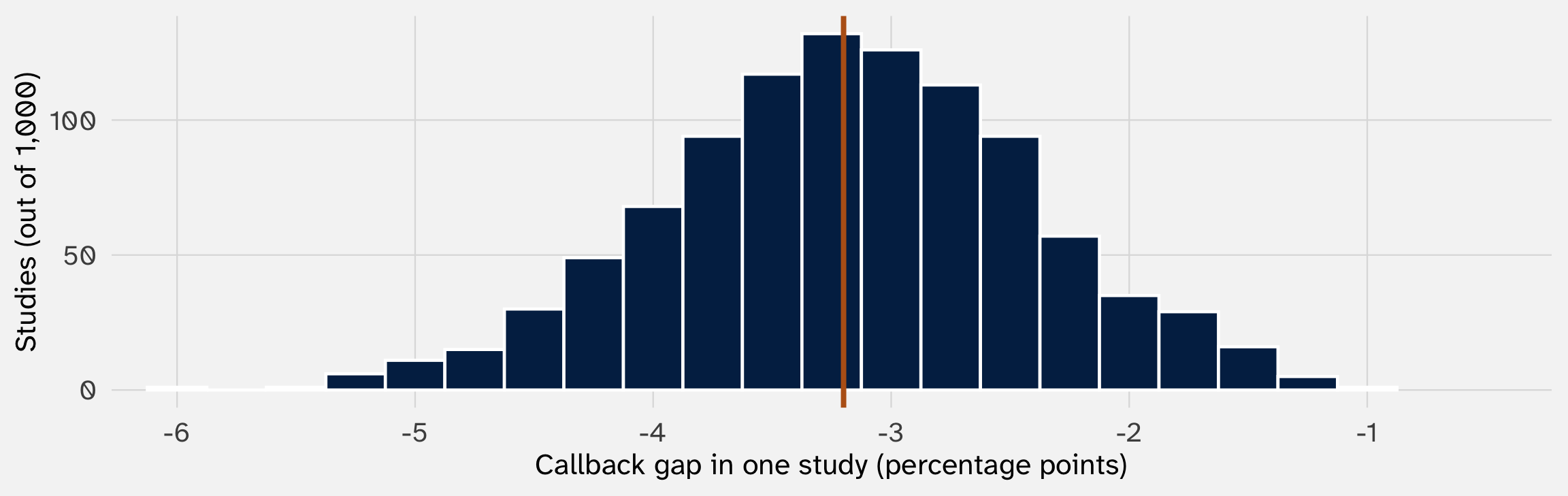
Every effect the study could produce: the sampling distribution of the estimate. It centers on the −3.2 points we built in
The standard deviation of the sampling distribution is the standard error
# A tibble: 1 × 2
   center  spread
    <dbl>   <dbl>
1 -0.0318 0.00776
A typical study lands about 0.8 points from the truth (−3.2).
In words: an AA-sounding name costs about 3 points of callback chance, give or take 0.8
The standard deviation of a sampling distribution is the standard error of the estimate. It’s the number in parentheses in every regression table, including week 1’s
What if our study had been smaller (N = 500)?
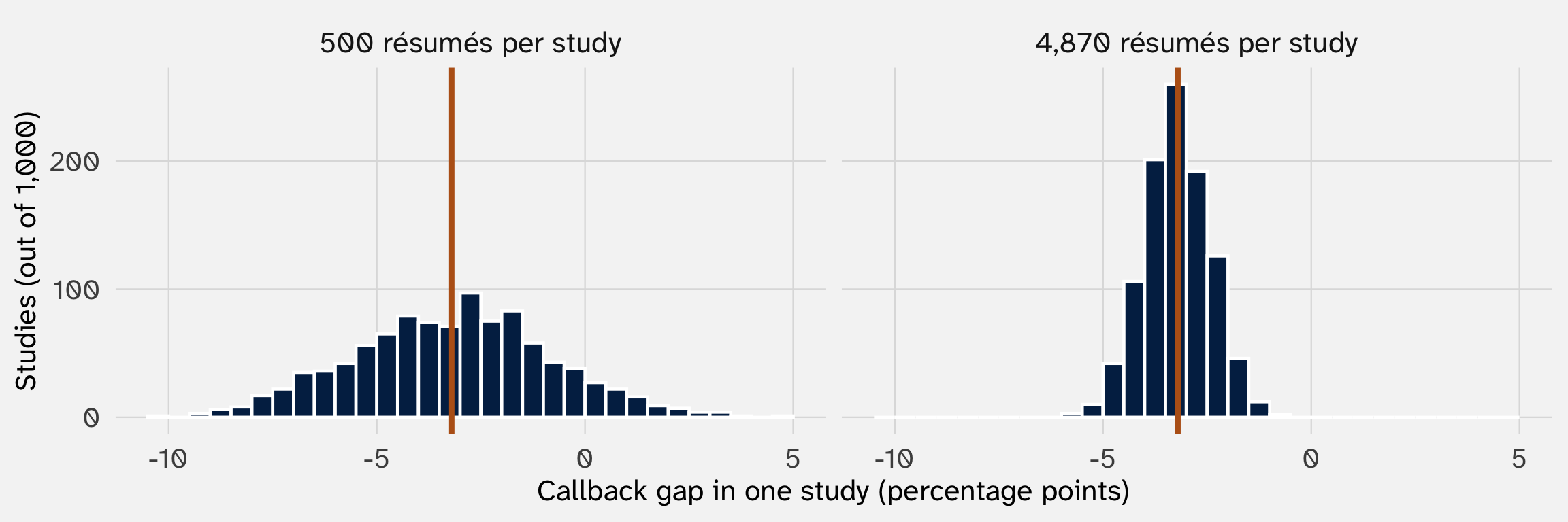
With 500 résumés the standard error is 2.4 points, against 0.8 with 4,870
Simulation shows that the sampling distribution depends on the size of the study
Week 3 we saw the standard error formula
We can simulate the standard error, or arrive at it analytically (math, proofs)
Week 3: the standard error is built from each group’s variance and size
\[ SE = \sqrt{\frac{\text{Var}_{\text{AA}}}{n_{\text{AA}}} + \frac{\text{Var}_{\text{white}}}{n_{\text{white}}}} = 0.0078 \]
| Callback (1) | |
|---|---|
| African American-sounding name | -0.032 |
| (0.0078) | |
| Intercept | 0.097 |
| (0.0055) | |
| Résumés | 4,870 |
Linear regression. Outcome: callback = 1 if the employer called back, 0 if not. Standard errors in parentheses.
Today we’ll see how to derive this formula
Recap: a random variable is a number we haven’t seen yet
An experiment is one run of a random process: send one résumé to one employer. Its sample space is every outcome that could happen: \(\{\text{callback}, \text{no callback}\}\)
A random variable translates outcomes into numbers: \(Y = 1\) for a callback, \(0\) for none. Before the employer decides, \(Y\) could be either. Once they decide, we see data: \(y = 0\)
| Written | What it is | |
|---|---|---|
| Random variable | \(Y\) | The number before the DGP produces it: it could be 0 or 1 |
| Data | \(y\) | The number the DGP produced this time |
One random variable per résumé: \(Y_1, Y_2, \ldots, Y_n\). The subscript says whose coin flip. Each has its own distribution (its own \(p_i\)); why?
The estimate is a random variable too. Before the study ran, \(\hat{\Delta}\) could have come out −1 point, −3, −5. The −3.2 is the one value it took
Recap: a probability distribution says how likely each value is
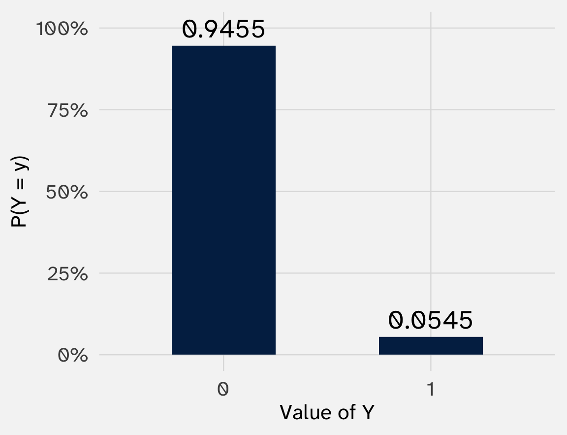
Résumé #1 from last week’s DGP had \(p_1\) = 0.0545:
\[ P(Y_1 = 1) = 0.0545, \qquad P(Y_1 = 0) = 0.9455 \]
Every value \(Y_1\) can take, and how likely each is. For a 0/1 outcome that’s the Bernoulli distribution, \(Y_1 \sim \text{Bernoulli}(p_1)\), with one parameter
\(p_1\) is a setting on the DGP: last week’s systematic part wrote it down. In real data we never see \(p\). We see outcomes, and from them a share, \(\hat{p}\)
Today asks two things about any distribution: where is it centered, and how spread out is it? For data, the mean and the variance. For a random variable, it’s the expectation and the variance
Today
- Center: why the sampling distribution centers on the truth
- Spread: how much one coin flip varies, then a callback share, then the gap
- The payoff: week 1’s standard error from one run of data
The gap is built out of smaller random variables
We want to know the center and spread of the gap’s sampling distribution. The gap itself is a difference of two shares:
\[ \hat{\Delta} = \hat{p}_{\text{AA}} - \hat{p}_{\text{white}} \]
Each share is an average of coin flips, one per résumé in that group:
\[ \hat{p}_{\text{AA}} = \frac{Y_1 + Y_2 + \cdots + Y_n}{n} \]
And each coin flip is a simple random variable: \(Y_i \sim \text{Bernoulli}(p_i)\), a 1 with chance \(p_i\)
If we can work out the center and spread of (say) \(Y_1\), we can work out the center and spread of \(\hat{\Delta}\)
We’ll fill this table in from top to bottom
| Center: \(E[\,\cdot\,]\) | Spread: \(\text{Var}(\,\cdot\,)\) | |
|---|---|---|
| One coin flip (an AA résumé), \(Y_i\) | ? | ? |
| A callback share, \(\hat{p}_{\text{AA}}\) | ? | ? |
| The gap, \(\hat{\Delta}\) | ? | ? |
Start with \(Y_i\), its center and spread
Then: what happens to the center and the spread when we average many coin flips? And when we subtract two averages?
Finally: the bottom-right cell is the variance of the gap. Its square root is week 1’s 0.0078
Where is the sampling distribution centered?
A random variable has no data yet. So what’s its “average”?
Week 3: the mean of data adds up the values and divides by \(n\)
A random variable is a number we haven’t seen yet. But we know every value it could take and how likely each is: its distribution
The expected value weights each possible value by its probability:
\[ E[X] = \sum_{x} x \cdot P(X = x) \]
A weighted average (week 3), with probabilities as the weights. The center of the distribution is where the draws would average out over many runs
The expected value of a coin flip is its probability
Résumé #1 from last week (AA-sounding name, 6 years of experience, age 49, 23 miles away) had \(p_1\) = 0.0545:
\[ E[X] = \sum_{x} x \cdot P(X = x) \]
\[ E[Y_1] = 1 \cdot P(Y_1 = 1) + 0 \cdot P(Y_1 = 0) = 1 \cdot p_1 + 0 \cdot (1 - p_1) = p_1 = 0.0545 \]
For any Bernoulli: \(E[Y] = p\). The expected value of a 0/1 variable is the chance it’s a 1
Remember: \(E[Y_1]\) is 0.0545, a value \(Y_1\) can never take. The expectation is the center of the distribution, not a typical draw
Check it by simulation: the long-run average of draws is the expectation
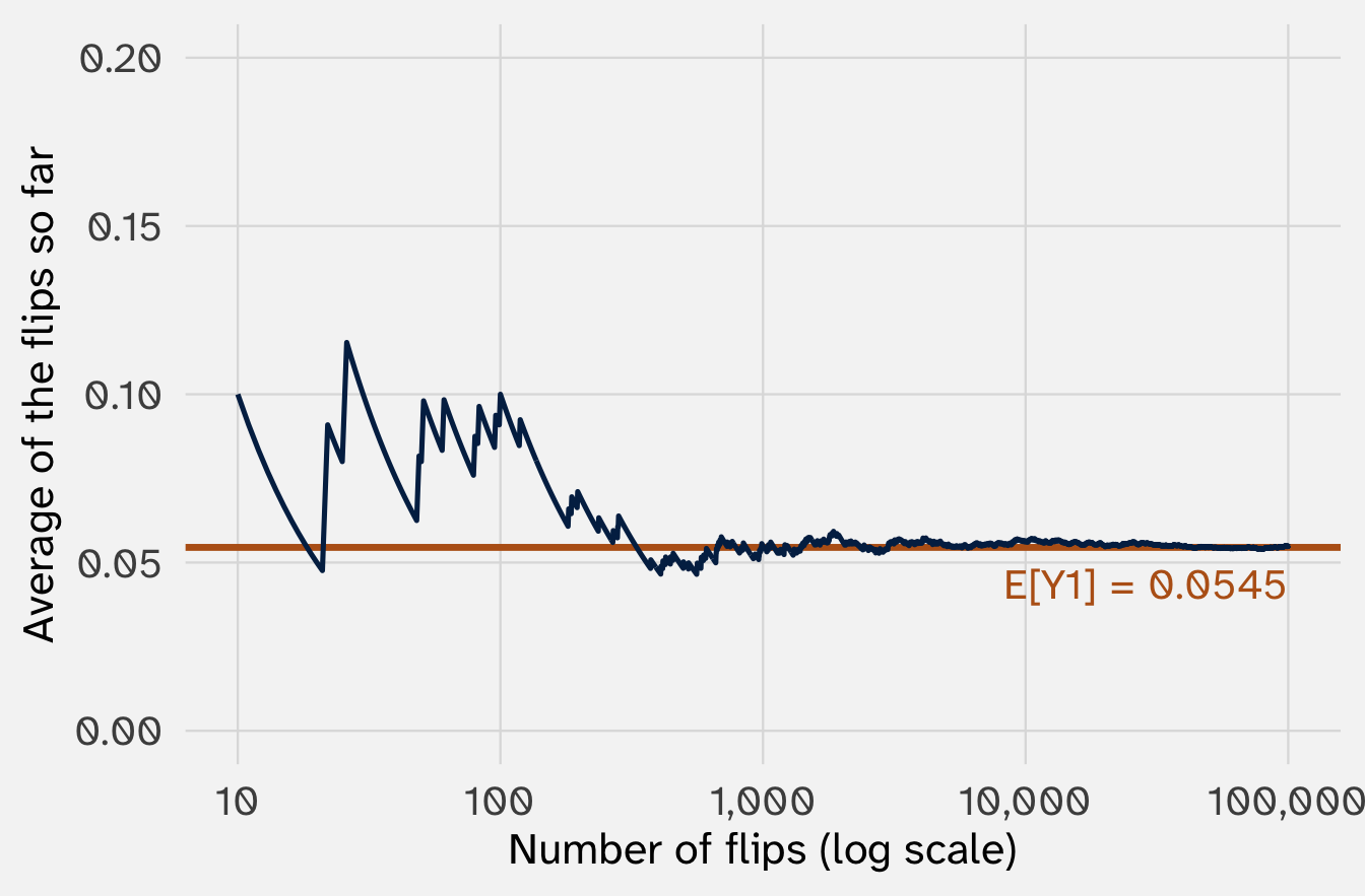
The analytic answer: \(E[Y_1] = p_1 = 0.0545\). That’s what the expectation means: early on the average swings around, but run the process over and over and it settles on \(E[X]\)
The expectation is the best guess, in the week 3 sense
Week 3: the mean is the guess that minimizes mean squared error in data
The same is true for a random variable: \(E[X]\) is the guess \(g\) that minimizes the expected squared miss, \(E[(X - g)^2]\)
So the expectation is to a random variable what the mean is to data: the center, and the best single guess
Expectation follows the same rules as the mean in week 3
| Week 3: the mean of data | Today: the expectation of a random variable |
|---|---|
| Multiply every value by \(k\), and the mean is multiplied by \(k\) | \(E[kX] = k \, E[X]\) |
| Add \(k\) to every value, and the mean moves by \(k\) | \(E[X + k] = E[X] + k\) |
| The mean of a constant is the constant | \(E[k] = k\) |
| Add/subtract two columns, and their means add/subtract | \(E[X + Y] = E[X] + E[Y]\) |
Why we need these: the callback share is a sum of coin flips divided by \(n\)
\[ \hat{p}_{\text{AA}} = \frac{Y_1 + Y_2 + \cdots + Y_n}{n} \]
The most important rule: the expectation of a sum is the sum of the expectations
\[ E[X + Y] = E[X] + E[Y] \]
Always. It doesn’t matter whether \(X\) and \(Y\) are related, how they’re distributed, or anything else
So:
\[E[Y_1 + Y_2 + \dots + Y_n] = E[Y_1] + E[Y_2] + \dots + E[Y_n]\]
Let’s convince ourselves this is true
Your turn: the expected sum of two dice
Roll two fair dice, \(D_1\) and \(D_2\)
- By hand: \(E[D_1]\), \(E[D_2]\), and \(E[D_1 + D_2]\)
- Simulate 100,000 rolls of each die with
sample(1:6, size = 100000, replace = TRUE). Ismean(d1 + d2)close? - The rule says “always,” even when the two numbers are related. Roll one die and count it twice: d1 + d1. Is \(E[D_1 + D_1]\) still \(E[D_1] + E[D_1]\)?
Remember: the expected value is the center of the distribution
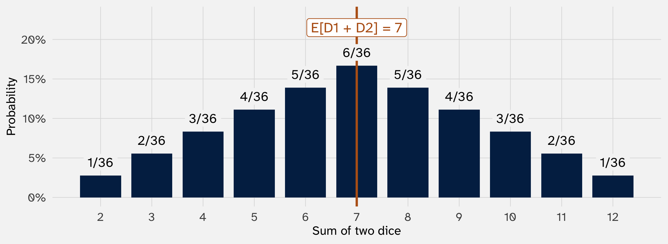
The sum can be anything from 2 to 12. Its expectation, 7, sits at the center: the balance point of the distribution, where the rolls average out over many tries
Payoff 1: the callback share is centered on the callback chance
The share of résumés with an AA-sounding name called back (below). What is the expectation of \(\hat{p}_{\text{AA}}\)? And what does that mean?
\[ \hat{p}_{\text{AA}} = \frac{Y_1 + Y_2 + \cdots + Y_n}{n} \]
Its expectation, one rule at a time:
\[ E[\hat{p}_{\text{AA}}] = \frac{1}{n} E[Y_1 + \cdots + Y_n] = \frac{1}{n} \left(E[Y_1] + \cdots + E[Y_n]\right) = \frac{1}{n} \cdot n \, p_{\text{AA}} = p_{\text{AA}} \]
Pull out the \(1/n\) (constant rule), split the sum (sum rule), each flip has expectation \(p_{\text{AA}}\) (Bernoulli).
What it means: rerun the study many times, and the share called back averages out to \(p_{\text{AA}}\), the true chance of a call. Any one run can land above or below it, but not systematically
What if \(p_i\) differ?
In last week’s DGP, each résumé had its own chance of a call, \(p_i\), set by its experience, age, and distance. The math works the same way, and the share is centered on the average \(p_i\) among AA-named résumés. From here on, \(p_{\text{AA}}\) means that average
Check it: the share centers on the average \(p_i\)
[1] 0.06373534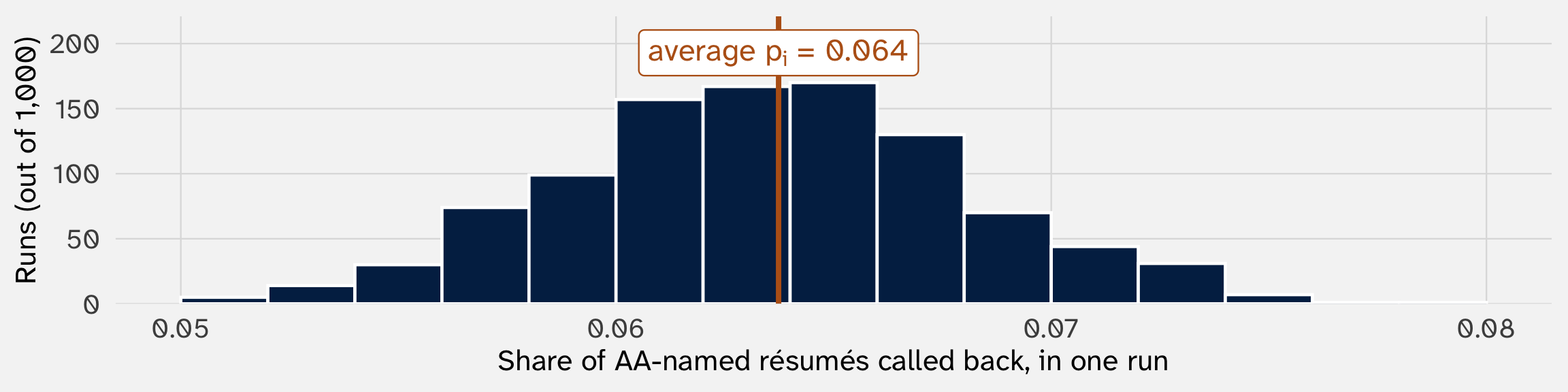
The \(p_i\) run from 0.023 to 0.107. The 1,000 shares average 0.0635; the average \(p_i\) is 0.0637
Payoff 2: the estimator is centered on the gap in callback chances
The estimator from week 1 is a difference of two shares:
\[ \hat{\Delta} = \hat{p}_{\text{AA}} - \hat{p}_{\text{white}} \]
The sum rule works for differences too (\(X - Y\) is \(X + (-1) \cdot Y\)):
\[ E[\hat{\Delta}] = E[\hat{p}_{\text{AA}}] - E[\hat{p}_{\text{white}}] = p_{\text{AA}} - p_{\text{white}} = \Delta \]
On average across reruns, the difference in means lands on the true gap in callback chances between the two groups
We say the estimator is unbiased for that gap
Unbiased for the gap or the effect?
Be very careful! This is one area where overlapping terminology (bias) is confusing
This shows that the estimator is an unbiased estimate of the gap between the two groups:
\[ E[\hat{\Delta}] = E[\hat{p}_{\text{AA}}] - E[\hat{p}_{\text{white}}] = p_{\text{AA}} - p_{\text{white}} = \Delta \]
Whether that gap is causal is a separate question; in the experiment, it’s established by randomization
What if we hadn’t randomized, and résumés with AA names tended to have less experience?
Only randomization makes the gap the effect
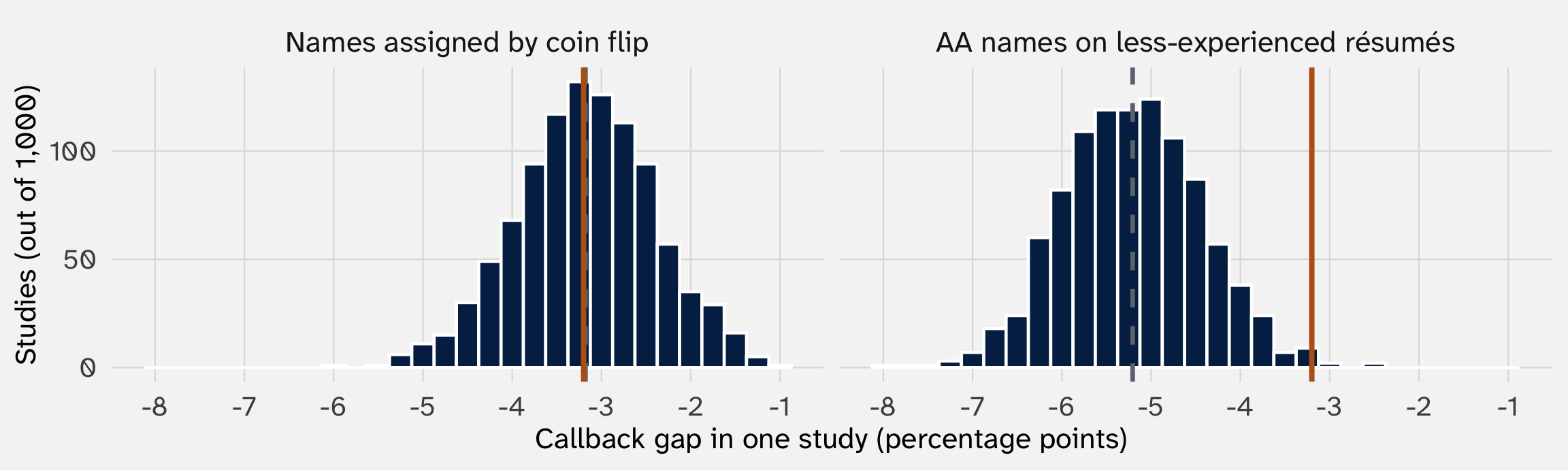
Orange: the effect of the name, −3.2 in both worlds. Dashed: where each sampling distribution centers, the gap between the groups. Both designs are unbiased for that gap. Only randomization makes the gap the effect. That’s confounding, from week 2
Unbiased is the first of four things an estimator can be
| Property | What it means | Where it comes up |
|---|---|---|
| Unbiased | Its sampling distribution is centered on the estimand | Today (Payoff 2) |
| Consistent | It lands ever closer to the estimand as \(n\) grows | Week 6 (the law of large numbers); named in week 7 |
| Asymptotically normal | Its sampling distribution is bell-shaped once \(n\) is large | Week 6 (the central limit theorem) |
| Efficient | Among unbiased estimators, the one with the smallest spread | Week 7 (several estimators of the same mean, compared) |
The center column is done: every row is centered on its target
| Center: \(E[\,\cdot\,]\) | Spread: \(\text{Var}(\,\cdot\,)\) | |
|---|---|---|
| One coin flip (an AA résumé), \(Y_i\) | \(p_{\text{AA}}\) | ? |
| A callback share, \(\hat{p}_{\text{AA}}\) | \(p_{\text{AA}}\) | ? |
| The gap, \(\hat{\Delta}\) | \(\Delta = p_{\text{AA}} - p_{\text{white}}\) | ? |
Question 1 answered. Now the spread column, starting with one coin flip
Let’s take a 10-minute break
How much does one coin flip vary?
The variance of a random variable is the expected squared miss
Week 3: the variance of data is the average squared distance from the mean
\[ \text{Var}(Y) = \frac{1}{n} \sum_{i=1}^{n} (Y_i - \bar{Y})^2 \]
For a random variable, replace the average with an expectation, and the mean with \(E[X]\):
\[ \text{Var}(X) = E\!\left[(X - E[X])^2\right] \]
And an expectation is a probability-weighted average, so we compute it the same way as \(E[X]\): take each possible squared miss, weight it by how likely it is, and add
\[ \text{Var}(X) = \sum_{x} (x - E[X])^2 \cdot P(X = x) \]
How far a draw typically lands from the center, squared. The standard deviation is its square root, \(\sigma = \sqrt{\text{Var}(X)}\), back in the variable’s units
A coin flip’s variance is \(p(1 - p)\)
Use the recipe from the last slide. A coin flip can miss its center \(p\) in only two ways:
| Outcome | Miss from \(p\) | Squared miss | Probability |
|---|---|---|---|
| \(Y = 1\) | \(1 - p\) | \((1 - p)^2\) | \(p\) |
| \(Y = 0\) | \(-p\) | \(p^2\) | \(1 - p\) |
Each row’s squared miss times its probability, added up:
\[ \text{Var}(Y) = \underbrace{(1 - p)^2 \cdot p}_{Y = 1} + \underbrace{p^2 \cdot (1 - p)}_{Y = 0} = p(1 - p)\left[(1 - p) + p\right] = p(1 - p) \]
For résumé #1 (\(p = 0.0545\)): \(p_1 (1 - p_1)\) = 0.0515
In general, the variance of a Bernoulli random variable is \(\text{Var}(Y) = p(1 - p)\)
Rare outcomes have small variance: a callback is rare
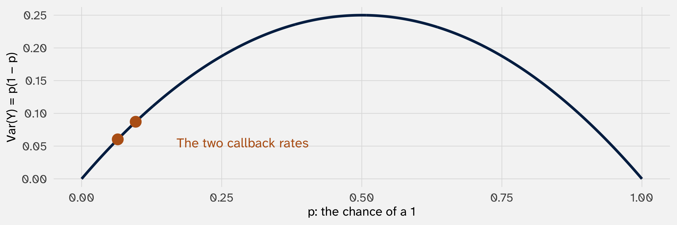
When is the variance highest? At \(p = 0.5\), a fair coin, and shrinks toward 0 as the outcome becomes nearly certain either way
Why is it intuitive that the variance of a résumé callback maxes out at \(p = 0.5\)?
Check it by simulation
# A tibble: 1 × 3
  average variance    sd
    <dbl>    <dbl> <dbl>
1  0.0548   0.0518 0.228
The analytic answers: \(E[Y_1]\) = 0.0545 and \(\text{Var}(Y_1)\) = 0.0515. Both are close
Variance has rules too
| Rule | In symbols | Why |
|---|---|---|
| Adding a constant doesn’t change the spread | \(\text{Var}(X + k) = \text{Var}(X)\) | Shifting every value shifts the center too; the misses don’t change |
| A constant has no spread | \(\text{Var}(k) = 0\) | It never misses |
| Multiplying by \(k\) multiplies the variance by \(k^2\) | \(\text{Var}(kX) = k^2 \, \text{Var}(X)\) | Every miss is \(k\) times bigger, and misses get squared |
| Adding two random variables | \(\text{Var}(X + Y) = \text{Var}(X) + \text{Var}(Y) + 2\,\text{Cov}(X, Y)\) | A third term for whether \(X\) and \(Y\) move together (covariance, week 3). More in a few slides |
| Subtracting one from another | \(\text{Var}(X - Y) = \text{Var}(X) + \text{Var}(Y) - 2\,\text{Cov}(X, Y)\) | Same pieces; only the covariance term flips sign |
Why we need these rules
The callback share divides a sum of coin flips by \(n\):
\[ \text{Var}(\hat{p}_{\text{AA}}) = \text{Var}\!\left(\frac{Y_1 + Y_2 + \cdots + Y_n}{n}\right) = \underbrace{\frac{1}{n^2}}_{k^2 \text{ rule}} \, \underbrace{\text{Var}(Y_1 + Y_2 + \cdots + Y_n)}_{\text{sum rule}} \]
The gap is a difference of two shares:
\[ \text{Var}(\hat{\Delta}) = \underbrace{\text{Var}(\hat{p}_{\text{AA}} - \hat{p}_{\text{white}})}_{\text{difference rule}} \]
So the \(k^2\) rule handles the \(n\), and the sum and difference rules handle the rest. Those two are the ones with the covariance term
Check the \(k^2\) rule by simulation
A fair coin: \(p = 0.5\), so \(\text{Var}(X) = 0.5 \times 0.5 = 0.25\). The rules say:
\[ \text{Var}(2X) = 2^2 \times 0.25 = 1 \qquad\qquad \text{Var}(X + 10) = \text{Var}(X) = 0.25 \]
# A tibble: 1 × 3
  var_x var_doubled var_shifted
  <dbl>       <dbl>       <dbl>
1 0.250        1.00       0.250
The simulation agrees: doubling the variable quadruples the variance (0.25 to 1), and shifting it by 10 does nothing
Your turn: a protest’s size as a random variable
A protest tomorrow will be small (100 people), medium (1,000), or large (10,000), with probabilities 0.6, 0.3, and 0.1
- By hand: \(E[X]\) and \(\text{Var}(X)\). (Make a table like the coin flip’s: value, probability, miss, squared miss)
- Simulate 100,000 protests with
sample(...). Domean()andvar()match your answers?
What’s left: how much do a share and the gap vary?
| Center: \(E[\,\cdot\,]\) | Spread: \(\text{Var}(\,\cdot\,)\) | |
|---|---|---|
| One coin flip (an AA résumé), \(Y_i\) | \(p_{\text{AA}}\) | \(p_{\text{AA}}(1 - p_{\text{AA}})\) |
| A callback share, \(\hat{p}_{\text{AA}}\) | \(p_{\text{AA}}\) | ? |
| The gap, \(\hat{\Delta}\) | \(\Delta = p_{\text{AA}} - p_{\text{white}}\) | ? |
The number we’re after is the variance of the gap. Its square root is week 1’s 0.0078:
\[ \text{Var}(\hat{\Delta}) = \text{Var}(\hat{p}_{\text{AA}} - \hat{p}_{\text{white}}) \]
Each share is a sum of \(n\) flips, divided by \(n\), and the gap is a difference of two shares. So both cells need the sum and difference rules, and both rules carry a term we haven’t explained: \(2\,\text{Cov}(X, Y)\)
What is \(\text{Cov}(X, Y)\) and what does it depend on?
How much does a share vary?
Where does the covariance term come from? Two résumés
Two résumés go out. \(Y_1\) and \(Y_2\) are whether each gets a call, each with chance 0.1
Scenario A: they go to two different employers, who each flip their own coin
Scenario B: they go to an employer who decides about the pair at once: call back both, or neither
Either way, the pair gets 0.2 callbacks on average: \(E[Y_1 + Y_2] = 0.1 + 0.1 = 0.2\)
But does the number of callbacks vary by the same amount? Is \(\text{Var}(Y_1 + Y_2)\) the same in both scenarios?
Linked coins vary twice as much
set.seed(211)
two = tibble(run = 1:100000) |>
  mutate(y1 = rbinom(n(), size = 1, prob = 0.1),      # résumé 1's call
         y2_own = rbinom(n(), size = 1, prob = 0.1),  # A: résumé 2 gets its own coin
         y2_same = y1)                                # B: résumé 2 gets the same coin
two |>
  summarize(mean_A = mean(y1 + y2_own), var_A = var(y1 + y2_own),
            mean_B = mean(y1 + y2_same), var_B = var(y1 + y2_same))
# A tibble: 1 × 4
mean_A var_A mean_B var_B
<dbl> <dbl> <dbl> <dbl>
1 0.201 0.180 0.201 0.361Same expectation (0.2). But the variance of the total is 0.18 with separate coins and 0.36 with one coin: twice as much
So \(\text{Var}(X + Y)\) is not just \(\text{Var}(X) + \text{Var}(Y)\). It depends on whether \(X\) and \(Y\) move together, depend on one another, or covary
“Moving together” = covariance
Week 3: the covariance of two variables in data asks whether they miss their averages together
\[ \text{Cov}(X, Y) = \frac{1}{n} \sum_{i=1}^{n} (X_i - \bar{X})(Y_i - \bar{Y}) \]
Same recipe as the variance: replace the average with an expectation, and the means with \(E[X]\) and \(E[Y]\)
\[ \text{Cov}(X, Y) = E\!\left[(X - E[X])(Y - E[Y])\right] \]
- Positive: when \(X\) is above its center, \(Y\) tends to be too (the same coin: both call or neither)
- Zero: \(X\) above its center tells you nothing about \(Y\) (separate coins)
- Negative: when one is high, the other tends to be low
The rule: the variance of a sum has a third term
\[ \text{Var}(X + Y) = \text{Var}(X) + \text{Var}(Y) + 2 \, \text{Cov}(X, Y) \]
The sum row of the rules table, from a few slides back. Now we can see what the third term does
Back to the two résumés. Each is a coin flip with \(p = 0.1\), so each has variance \(p(1 - p) = 0.1 \times 0.9 = 0.09\):
| \(\text{Cov}(Y_1, Y_2)\) | \(\text{Var}(Y_1 + Y_2)\) | Simulation said | |
|---|---|---|---|
| A: separate coins | 0: the coins don’t move together | \(0.09 + 0.09 + 0 = 0.18\) | 0.18 |
| B: the same coin | 0.09: one coin moves perfectly with itself | \(0.09 + 0.09 + 2(0.09) = 0.36\) | 0.36 |
The third term is where “moving together” enters. When it’s zero, variances simply add, like expectations do
What would it mean for two résumés’ callbacks to covary?
Bertrand and Mullainathan sent four résumés to each job ad, so résumés really did share employers (Bertrand and Mullainathan 2004)
Scenario B was the extreme: one decision for the pair. A real employer still makes a separate call on each résumé (week 4: rerun the same morning, and the manager might decide differently). What résumés at the same employer share is part of the chance:
- Positive covariance: an employer who badly needs to hire raises the chance for all four; one who already filled the job lowers it for all four
- Negative covariance: an employer with a single interview slot calls back at most one. If résumé 1 got the call, résumé 2 probably didn’t
- Zero covariance: résumés sent to different employers with nothing in common
So a shared employer gives some covariance, but less than scenario B’s
Independent: one résumé’s call tells you nothing about the other’s
Conditional probability, \(P(A \mid B)\): the chance of \(A\) given \(B\). Among the runs where résumé 1 got a call, how often did résumé 2 get one?
\(X\) and \(Y\) are independent when knowing one changes nothing about the other:
\[ P(Y = y \mid X = x) = P(Y = y) \qquad \text{for every } x \text{ and } y \]
Scenario A: résumé 2’s chance is 0.1 whether or not résumé 1 got a call. Scenario B: once résumé 1 got a call, résumé 2’s is certain
Independent variables have zero covariance, so their variances simply add.
Today’s standard error assumes the résumés are independent. Four résumés per ad strains that, and week 10 (clustering) deals with it
With more than two variables, every pair adds a covariance term
\[ \text{Var}(Y_1 + Y_2 + Y_3) = \text{Var}(Y_1) + \text{Var}(Y_2) + \text{Var}(Y_3) + 2\,\text{Cov}(Y_1, Y_2) + 2\,\text{Cov}(Y_1, Y_3) + 2\,\text{Cov}(Y_2, Y_3) \]
In general: one variance term for each variable, and one covariance term for each pair
\[ \text{Var}\!\left(\sum_{i=1}^{n} Y_i\right) = \sum_{i=1}^{n} \text{Var}(Y_i) + 2 \sum_{i < j} \text{Cov}(Y_i, Y_j) \]
The 2,435 AA résumés have 2,435 variance terms and 2,963,395 covariance terms. If the résumés are independent, every covariance term is zero, and the variance of the sum is just the sum of the variances
Payoff 3: the variance of an average shrinks with \(n\)
\(n\) independent flips, each with variance \(p_{\text{AA}}(1 - p_{\text{AA}})\). The callback share \(\hat{p}_{\text{AA}}\) is their sum over \(n\):
\[ \text{Var}(\hat{p}_{\text{AA}}) = \frac{1}{n^2} \, \text{Var}(Y_1 + \cdots + Y_n) = \frac{1}{n^2} \left[\text{Var}(Y_1) + \cdots + \text{Var}(Y_n)\right] = \frac{1}{n^2} \cdot n \, p_{\text{AA}}(1 - p_{\text{AA}}) = \frac{p_{\text{AA}}(1 - p_{\text{AA}})}{n} \]
Pull out \(1/n^2\) (\(k^2\) rule), split the sum (independence: no covariance terms), each flip has the same coin-flip variance (Bernoulli)
Its standard deviation is the standard error of the share:
\[ SE(\hat{p}_{\text{AA}}) = \sqrt{\frac{p_{\text{AA}}(1 - p_{\text{AA}})}{n}} \]
The same rule for any average: \(\text{Var}(\bar{X}) = \sigma^2 / n\)
The coin flip was a special case. For any outcome with variance \(\sigma^2\), the average of \(n\) independent draws has
\[ \text{Var}(\bar{X}) = \frac{\sigma^2}{n}, \qquad SE(\bar{X}) = \frac{\sigma}{\sqrt{n}} \]
Two things make an estimate vary (week 3’s note, now proved): noisy outcomes (big \(\sigma^2\)) and small samples (small \(n\))
How much does the gap vary?
Payoff 4: the standard error of the gap
The gap is a difference of two shares. The difference rule (last row of the rules table), with zero covariance because the two groups’ résumés are independent:
\[ \text{Var}(\hat{\Delta}) = \text{Var}(\hat{p}_{\text{AA}}) + \text{Var}(\hat{p}_{\text{white}}) = \frac{p_{\text{AA}}(1 - p_{\text{AA}})}{n_{\text{AA}}} + \frac{p_{\text{white}}(1 - p_{\text{white}})}{n_{\text{white}}} \]
Take the square root, and it’s week 3’s formula. Every piece now has a rule behind it:
\[ SE(\hat{\Delta}) = \sqrt{ \frac{\overbrace{p_{\text{AA}}(1 - p_{\text{AA}})}^{\text{coin-flip variance}}}{\underbrace{n_{\text{AA}}}_{\text{averaging independent flips}}} \overbrace{+}^{\text{independent shares}} \frac{p_{\text{white}}(1 - p_{\text{white}})}{n_{\text{white}}} } \]
A skeptic: the formula wants \(p\), but all we have is \(\hat{p}\)
The formula needs the true chances, \(p_{\text{AA}}\) and \(p_{\text{white}}\). Those are settings on the DGP, and the real study never shows them to us
So we plug in the shares from the data, \(\hat{p}\). That makes our standard error itself an estimate, from one run, with its own study-to-study variation
Why trust this estimate? \(\hat{p}\) lands close to \(p\) when \(n\) is large (Payoff 3: its variance shrinks with \(n\)). Why that’s guaranteed, and how close is “close”, is weeks 6 and 7
Plug in the one run we have
| Name on résumé | \(n\) | \(\hat{p}\) | \(\hat{p}(1 - \hat{p})\) | \(\hat{p}(1 - \hat{p}) / n\) |
|---|---|---|---|---|
| White-sounding | 2,435 | 0.0965 | 0.0872 | 0.0000358 |
| AA-sounding | 2,435 | 0.0645 | 0.0603 | 0.0000248 |
\[ SE(\hat{\Delta}) = \sqrt{\frac{0.0603}{2,435} + \frac{0.0872}{2,435}} = \mathbf{0.0078} \]
Three paths, one number
| Path | What it needed | \(SE(\hat{\Delta})\) |
|---|---|---|
| Simulation (week 4): the SD of 1,000 reruns | A DGP we built, with the truth set to −3.2 | 0.0078 |
| Analytic (today): \(\sqrt{\hat{p}(1-\hat{p})/n + \hat{p}(1-\hat{p})/n}\) | One run of the real data | 0.0078 |
Week 1’s table: lm() |
One run of the real data | 0.0078 |
The sampling distribution Bertrand and Mullainathan never saw has a standard error of about 0.78 points. Their −3.2 points is four standard errors from zero: not a fluke of which résumés got which names
One logic, a family of formulas
| Estimand | Estimator | Standard error |
|---|---|---|
| A mean | \(\bar{Y}\) | \(\sqrt{\sigma^2 / n}\) |
| A proportion | \(\hat{p}\) | \(\sqrt{p(1 - p) / n}\) |
| A difference in means | \(\bar{Y}_1 - \bar{Y}_0\) | \(\sqrt{\sigma_1^2 / n_1 + \sigma_0^2 / n_0}\) |
| A difference in proportions (the résumés) | \(\hat{p}_1 - \hat{p}_0\) | \(\sqrt{p_1(1 - p_1) / n_1 + p_0(1 - p_0) / n_0}\) |
Every row is the same three rules: a variance in the numerator, \(n\) in the denominator, pieces added across independent groups. A regression coefficient’s standard error (POL 212) is the same logic with more algebra
In practice you won’t derive these by hand. The point is to know what a standard error is a statement about, and what makes it big or small: the outcome’s variance, and the amount of data
So what?
Every cell, filled in from one run of data and a few rules
| Center: \(E[\,\cdot\,]\) | Spread: \(\text{Var}(\,\cdot\,)\) | |
|---|---|---|
| One coin flip (an AA résumé), \(Y_i\) | \(p_{\text{AA}}\) | \(p_{\text{AA}}(1 - p_{\text{AA}})\) |
| A callback share, \(\hat{p}_{\text{AA}}\) | \(p_{\text{AA}}\) | \(p_{\text{AA}}(1 - p_{\text{AA}}) / n\) |
| The gap, \(\hat{\Delta}\) | \(\Delta = p_{\text{AA}} - p_{\text{white}}\) | \(\frac{p_{\text{AA}}(1 - p_{\text{AA}})}{n_{\text{AA}}} + \frac{p_{\text{white}}(1 - p_{\text{white}})}{n_{\text{white}}}\) |
One run of data, plus the rules for adding random variables, tells you how wide a distribution you can never see is
Next week: the shape of the sampling distribution
We know where the sampling distribution sits (the truth) and how wide it is (\(\sigma / \sqrt{n}\)). We don’t yet know its shape
Last week’s sampling distribution looked like a bell. Next week: why every average looks like that when \(n\) is large (the central limit theorem), and what the bell shape buys us
Then: what “four standard errors from zero” lets you say (weeks 8 and 9)
References
Bertrand, Marianne, and Sendhil Mullainathan. 2004. “Are Emily and Greg More Employable Than Lakisha and Jamal? A Field Experiment on Labor Market Discrimination.” American Economic Review 94(4): 991–1013. doi:10.1257/0002828042002561.
Imai, Kosuke, and Nora Webb Williams. 2022. Quantitative Social Science: An Introduction in Tidyverse. Princeton, NJ: Princeton University Press.
Xu, Yiqing. 2026. “Point Estimation.” https://github.com/xuyiqing/regression-lectures.
POL 211 · Fall 2026