Probability: what if we could do it all over again?
POL 211 · Week 4
Juan F. Tellez
University of California, Davis
October 20, 2026
Exam 1
Write your answers in your blue book
Let’s take a 10-minute break
Today
- Pretend we know the DGP Simulate the résumé study, then run it again
- Where does the uncertainty come from?
- Random variables and probability distributions: a language for the random part
- Find the estimate’s distribution: rerun the study 1,000 times
If we ran the world again, would we get the same answer?
Reminder: the standard error from Week 1’s table
| Callback (1) | |
|---|---|
| African American-sounding name | -0.032 |
| (0.0078) | |
| Intercept | 0.097 |
| (0.0055) | |
| Résumés | 4,870 |
Linear regression. Outcome: callback = 1 if the employer called back, 0 if not. Standard errors in parentheses.
The estimated treatment effect, -3.2pp: how much less likely AA-sounding names to receive callback than White-sounding names
The standard error, 0.0078, is “how much the estimate would vary if we ran the study again.”
Today: how to think about why the estimate varies
Why would we get a different answer?
Week 1: our data are one run of a process
The résumé study found AA-sounding names got about 3 points fewer callbacks
Send the same résumés out again, to a fresh batch of employers, and we’d get a different number. Maybe 2.5 points. Maybe 4
This is because the Data-Generating Process (DGP) has a random component
Probability is the language for the random part: how much would the answer change if we ran the world again?
Suppose we knew exactly how employers decide
Let’s generate data from a DGP we control completely
The systematic part: each résumé’s chance of a call, \(p_i\)
- More experience: more calls
- Older: fewer calls
- Lives farther from the job: fewer calls
- Black-sounding name: fewer calls (our study)
The random part: each employer then flips a coin weighted by \(p_i\)
Step 1, the systematic part: each résumé’s chance of a call
set.seed(211)
resumes = tibble(name = sample(c("white", "black"), size = 4870, replace = TRUE),  # a coin flip picks each name
                 exper = sample(0:10, size = 4870, replace = TRUE),       # years of experience
                 age = sample(22:55, size = 4870, replace = TRUE),
                 distance = sample(0:30, size = 4870, replace = TRUE)) |> # miles from the job
  mutate(p = 0.099 - 0.032 * (name == "black") +   # Black-sounding name: -3.2 points
               0.004 * exper -                      # each year of experience: +0.4 points
               0.0005 * (age - 22) -                # each 10 years older: -0.5 points
               0.001 * distance)                    # each 10 miles away: -1 point
resumes
# A tibble: 4,870 × 5
name exper age distance p
<chr> <int> <int> <int> <dbl>
1 black 6 49 23 0.0545
2 white 4 23 23 0.0915
3 white 6 48 0 0.11
4 white 4 49 10 0.0915
5 black 0 41 0 0.0575
# ℹ 4,865 more rowsWe wrote \(p\) down ourselves: we know the systematic part exactly
Step 2, the random part: each employer flips a weighted coin
We want to turn those probabilities into call (0/1), where the probability that call = 1 depends on \(p\)
# A tibble: 4,870 × 6
  name  exper   age distance      p  call
  <chr> <int> <int>    <int>  <dbl> <int>
1 black     6    49       23 0.0545     0
2 white     4    23       23 0.0915     0
3 white     6    48        0 0.11       0
4 white     4    49       10 0.0915     0
5 black     0    41        0 0.0575     0
# ℹ 4,865 more rows
rbinom() flips one coin per résumé, each weighted by its own \(p\)
One run of the study gives one estimate
# A tibble: 2 × 2
  name  callback_rate
  <chr>         <dbl>
1 black        0.0680
2 white        0.0882
The difference in means: -2.0 points. The true gap we built in: −3.2
Run it again: same résumés, same \(p\)’s, new coin flips, a new estimate
# A tibble: 2 × 2
  name  callback_rate
  <chr>         <dbl>
1 black        0.0615
2 white        0.101
This time: -3.9 points. Even when we know exactly how the world works, and by how much, the estimate changes
Even with the systematic part known exactly, each résumé’s outcome is random
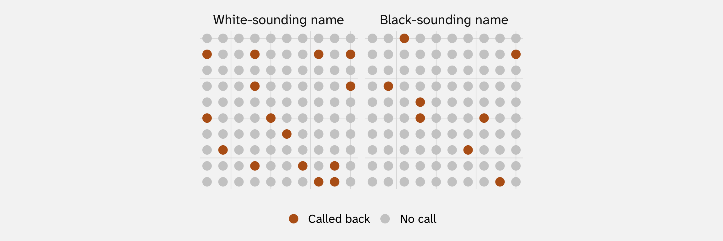
The name shifts the chance of a call. It doesn’t decide any one résumé: most résumés with either name get no call, and some Black-named résumés get calls that white-named ones don’t
The data give us \(\hat{p}\), not \(p\)
The callback rates we computed in runs 1 and 2 were \(\hat{p}\): shares in the data. The chances we wrote in Step 1 were \(p\). With real data, all we ever get is \(\hat{p}\):
\(p\) is a setting on the DGP: we never see it. \(\hat{p}\) (read “p-hat”) is the share in the one run we got: our estimate of \(p\)
Each run of the study is one turn of a machine
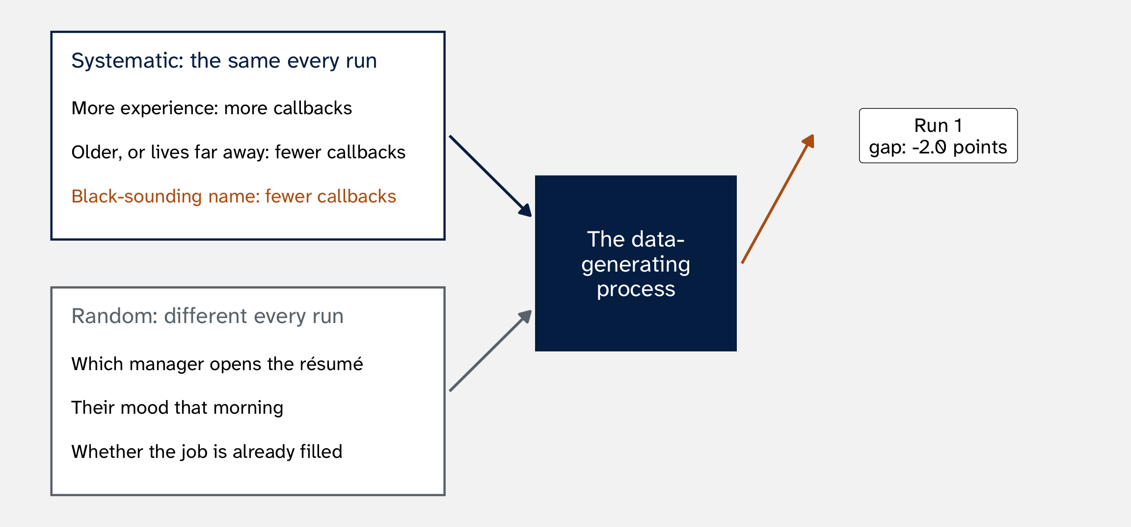
Turn it again: same systematic part, new random part, new answer
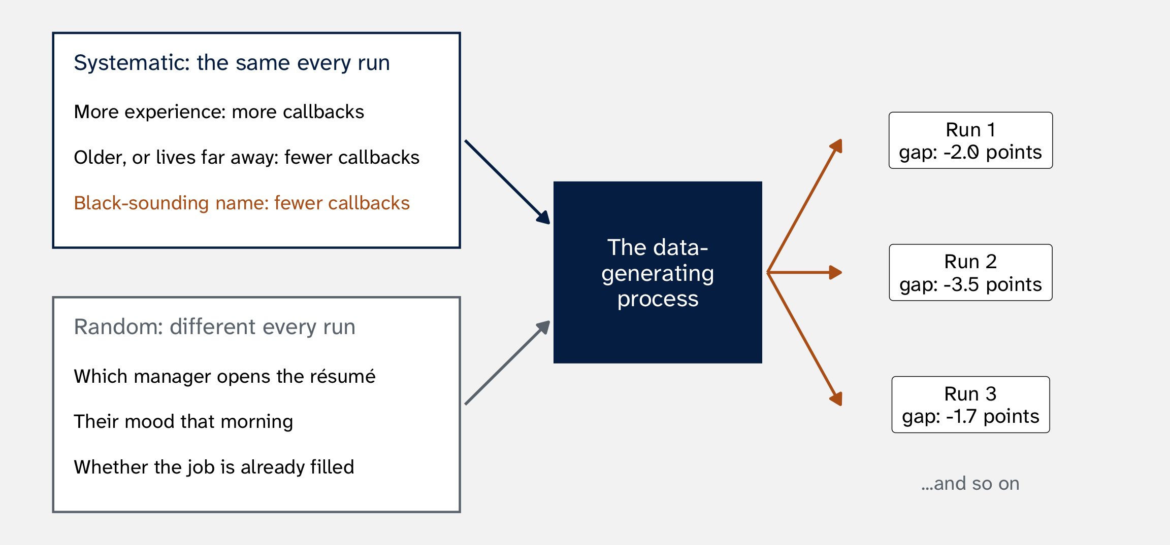
Where does that uncertainty come from? Randomness enters the data in three ways
| Source | What it means | In the résumé study |
|---|---|---|
| Sampling | We see only part of the whole | These employers, in these two cities, that year |
| Theoretical | Our theory leaves things out | The hiring manager’s mood that morning |
| Fundamental | People are partly random, even with a complete theory | Rerun the same morning, and the same manager might decide differently |
The three sources come from Gailmard (2014, 73–78)
Your turn: where does the uncertainty come from?
Which source is most at work: sampling, theoretical, or fundamental?
- A poll of 1,000 adults reports that 54% approve of the president
- A model of protest uses food prices and elections, but not the weather
- The same senator, on the same bill, might have voted the other way if the vote had been held a day later
- A city draws lottery numbers to decide which neighborhoods get new streetlights
The next few weeks: a language for this variation
We just watched the estimate change from run to run. The next few weeks build a mathematical language for that variation, so we can:
- describe it: the sampling distribution, every estimate the study could produce. Where is it centered, and what shape is it?
- measure it: how spread out that distribution is, the standard error (week 1’s 0.0078)
- say how uncertain to feel about the one estimate we actually get: confidence intervals and p-values
How can we describe how likely each outcome of a process is?
Random variables
Sending one résumé is an experiment; its possible outcomes are the sample space
An experiment is one run of a random process: send one résumé to one employer
The sample space, \(S\), lists every outcome that could happen:
\[ S = \{\text{callback}, \; \text{no callback}\} \]
(A die works the same way: roll it once, and \(S = \{1, 2, 3, 4, 5, 6\}\))
Sorry
Statistics, probability, and math are full of terribly overlapping concepts. This creates a lot of confusion
A random variable translates outcomes into numbers
The outcomes “callback” and “no callback” aren’t numbers. To do math with them, we translate:
\[ Y(\text{callback}) = 1, \qquad Y(\text{no callback}) = 0 \]
A random variable is that translation: a rule that turns each outcome in \(S\) into a number. We name random variables with capital letters
One hiring process, many possible random variables:
| Random variable | What it records |
|---|---|
| \(Y_i\) | Whether résumé \(i\) gets a callback |
| \(Z_i\) | How many days until the employer responds |
| \(W_i\) | Whether the employer offers an interview |
With random variables in hand, we can deploy concepts from statistics/probability to quantify uncertainty
A random variable is a number we haven’t seen yet
Before an employer opens résumé #1, we don’t know whether they’ll call. Call it \(Y_1\): it will turn out to be 1 (callback) or 0 (no callback)
Once they decide, we see data: \(y_1 = 0\)
| Written | What it is | |
|---|---|---|
| Random variable | \(Y\) | The number before the machine produces it: it could be 0 or 1 |
| Data | \(y\) | The number the machine produced this time |
This lets us make probability statements about \(Y_1\), like \(P(Y_1 = 1) = 0.05\)
but not about \(y_1\): once we’ve seen it, it’s just 0 or 1
Probability distributions
A probability distribution says how likely each value is
Definition: describes the probability of every possible outcome for a random variable
Résumé #1 from Step 1 (Black-sounding name, 6 years of experience, age 49, 23 miles away) got \(p_1\) = 0.0545:
\[ P(Y_1 = 1) = 0.0545, \qquad P(Y_1 = 0) = 0.9455 \]
Together, these are a probability distribution: every value \(Y_1\) can take, and how likely each one is
These are the true probabilities: settings on the DGP, known only because we built it in Step 1. With real data we never see them. We see outcomes: the empirical distribution, the real-life “footprint” of the true probability
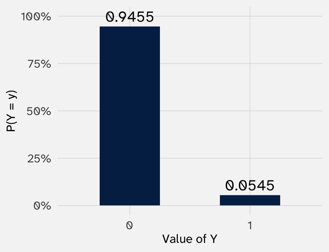
A 0/1 outcome has a Bernoulli distribution
\[ Y_i \sim \text{Bernoulli}(p_i) \]
Read it as: “\(Y_i\) is drawn from a Bernoulli with probability \(p_i\).” It takes the value 1 with probability \(p_i\) and 0 with probability \(1 - p_i\)
The formula:
\[ P(Y_i = y) = p_i^{\,y} \, (1 - p_i)^{1 - y}, \qquad y = 0 \text{ or } 1 \]
Plug in \(y = 1\): you get \(p_i\). Plug in \(y = 0\): you get \(1 - p_i\). One formula, both cases
One parameter: once we know \(p_i\), we know the whole distribution
rbinom()
This formula is what rbinom() draws from in Step 2
Other kinds of outcomes have other distribution families
| Type of outcome | Example | A distribution often used |
|---|---|---|
| Binary (0/1) | A callback | Bernoulli |
| Count | Number of protests in a week | Poisson |
| Continuous | Vote share; income | Normal (week 6); lognormal |
| Unordered categories | Democrat, Republican, independent | Categorical |
| Ordered categories | Strongly disagree … strongly agree | Ordered categorical |
Each family describes how probability is spread across the values an outcome can take, and each has parameters that set its shape. For anything beyond 0/1, picking the family is part of building the model
The systematic part lives inside \(p\): exactly what Step 1 did
- Pick a distribution whose outcomes look like ours. A callback is 0 or 1: the Bernoulli
- The systematic part lives in \(p_i\). It goes up with experience, and down with age, distance, and a Black-sounding name. That was Step 1
- The random part is the draw. Step 2’s coin flip stands in for everything we didn’t put in \(p_i\): moods, filled jobs, the causes we left out
\[ Y_i \sim \text{Bernoulli}(p_i), \qquad p_i = \text{baseline} - \text{Black name} + \text{experience} - \text{age} - \text{distance} \]
Estimand, estimator, estimate: week 2’s three terms, in symbols
| Term | In symbols | In the résumé study |
|---|---|---|
| Estimand | \(\Delta = p_{\text{Black}} - p_{\text{white}}\) | The true gap in callback chances: a setting on the machine |
| Estimator | \(\hat{p}_{\text{Black}} - \hat{p}_{\text{white}}\) | The rule: subtract the two callback shares |
| Estimate | \(\hat{\Delta}\) = -3.2 points | What the rule gave in the one run we saw (6.45% – 9.65%); the same number as week 1’s regression |
Before the data exist, the estimator’s answer is a random variable. The estimate is its realization: the \(y\) to its \(Y\)
Your estimate is a random variable too
Before Bertrand and Mullainathan ran their study, \(\hat{\Delta}\) was a random variable: built from 4,870 Bernoulli draws, it could have come out −1 point, −3 points, −5 points…
The −3.2 points they reported is one draw
And like any random variable, \(\hat{\Delta}\) has a distribution: every value the gap could take, and how often
The sampling distribution: every estimate the DGP could produce, and how often
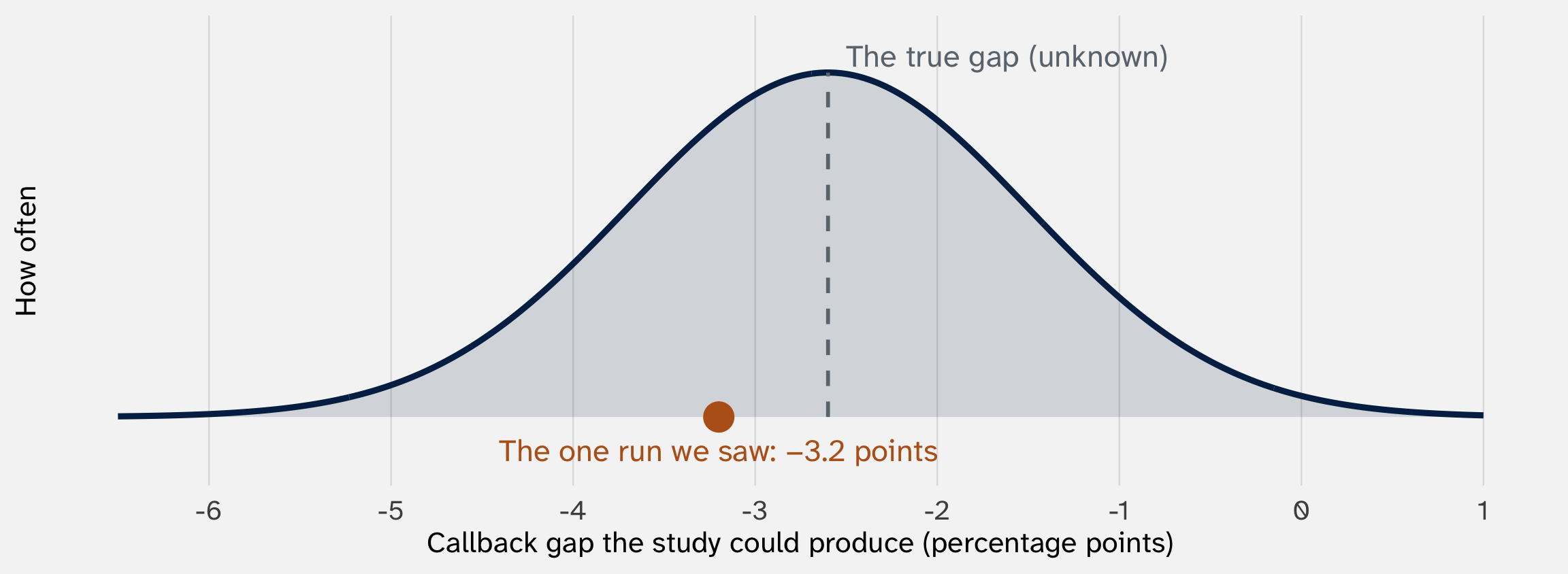
This is what the DGP would generate across many runs of the study. We never see it: Bertrand and Mullainathan ran once. It’s hypothetical
But we built this DGP, so we can see it
# the DGP from Steps 1 and 2
resumes = tibble(
  name = sample(c("white", "black"), size = 4870, replace = TRUE),
  exper = sample(0:10, size = 4870, replace = TRUE),
  age = sample(22:55, size = 4870, replace = TRUE),
  distance = sample(0:30, size = 4870, replace = TRUE)) |>
  mutate(
    # systematic: the same rule every run
    p = 0.099 - 0.032 * (name == "black") + 0.004 * exper -
        0.0005 * (age - 22) - 0.001 * distance,
    # random: new coin flips every run
    call = rbinom(4870, size = 1, prob = p))
All we have to do is run this code thousands of times, compute the gap each time, and pile up the gaps
Find the estimate’s distribution
Problem Set 3: you already wrote a function
A function takes inputs (here, a variable and a guess) and returns an output (here, a number)
Today: no inputs, and the output is a whole made-up dataset. The function is the data-generating process
Wrap the two steps in a function, so we can run the study with one line
make_resumes = function() {
  tibble(name = sample(c("white", "black"), size = 4870, replace = TRUE),
         exper = sample(0:10, size = 4870, replace = TRUE),
         age = sample(22:55, size = 4870, replace = TRUE),
         distance = sample(0:30, size = 4870, replace = TRUE)) |>
    mutate(p = 0.099 - 0.032 * (name == "black") + 0.004 * exper -
                 0.0005 * (age - 22) - 0.001 * distance,      # step 1: systematic
           call = rbinom(4870, size = 1, prob = p))            # step 2: random
}

run_resumes = function() {
  make_resumes() |>
    summarize(gap = mean(call[name == "black"]) - mean(call[name == "white"])) |>
    pull(gap)                                                    # just the estimate
}Rerun the study 1,000 times
# A tibble: 1,000 × 2
    run     gap
  <int>   <dbl>
1     1 -0.0202
2     2 -0.0354
3     3 -0.0168
4     4 -0.0305
5     5 -0.0321
# ℹ 995 more rows
One row per study. Each gap is a \(\hat{\Delta}\) the study could have produced
After 10 studies, no shape yet
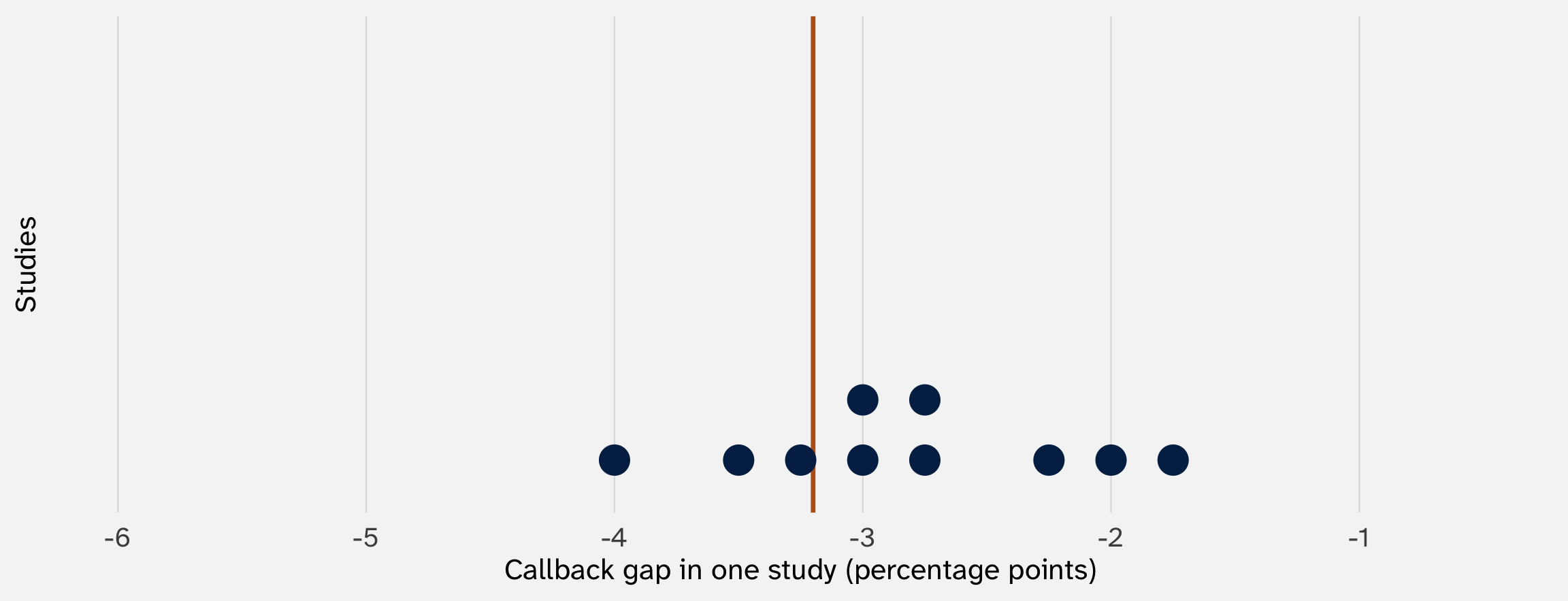
Each dot is one whole study. The orange line is the true gap we built in (−3.2 points)
After 100 studies, a shape appears
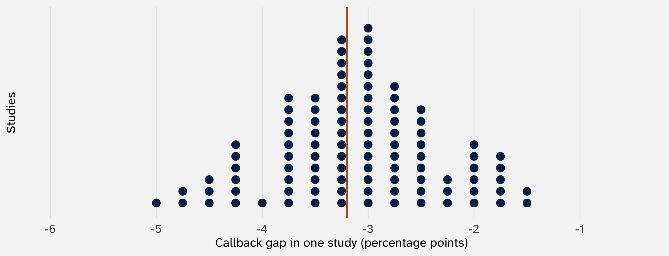
After 1,000 studies: we just simulated the sampling distribution
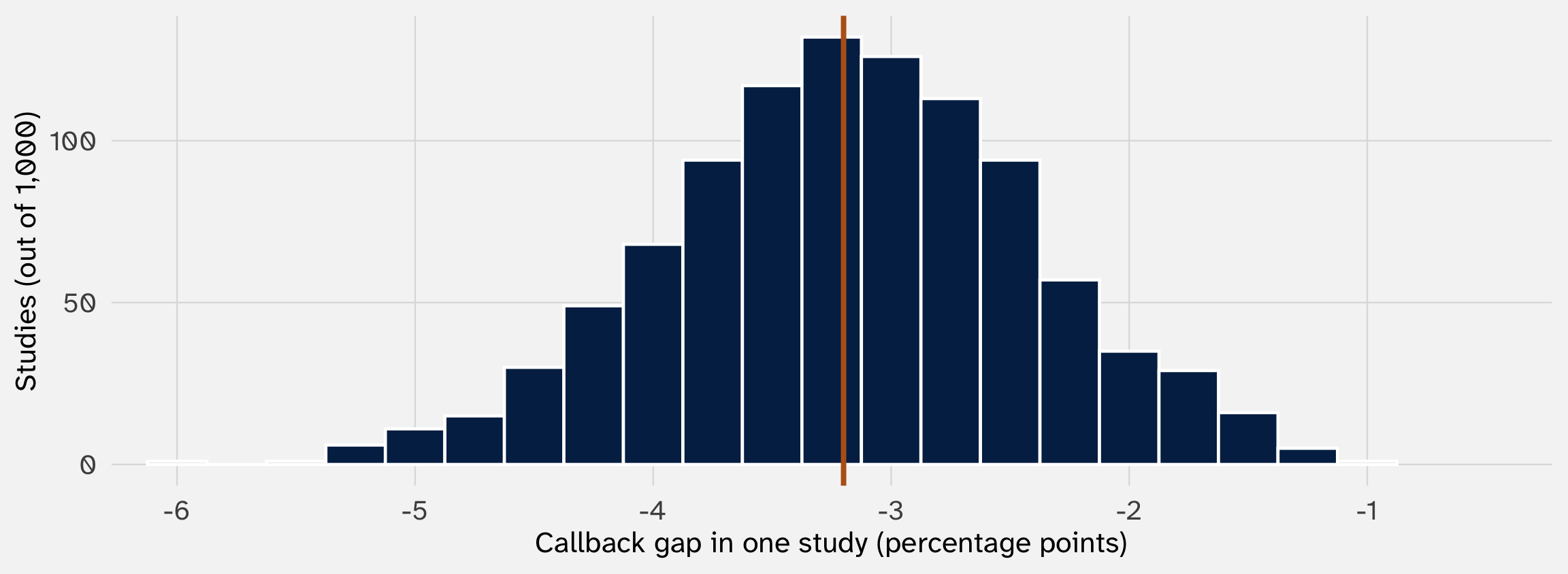
The hypothetical curve from before, made visible. What stands out? And how could we quantify how much the estimate bounces?
The pile centers on the truth, and its spread is a standard deviation
# A tibble: 1 × 2
  average_gap  spread
        <dbl>   <dbl>
1     -0.0318 0.00776
Center: the average of the 1,000 estimates is the −3.2 points we built in. The estimator is unbiased: it lands on the truth on average, though any one run can miss
Spread: the standard deviation of the 1,000 estimates says how far a typical run lands from the truth
Two ways to find a sampling distribution
1. Analytic
- Use formal rules of mathematics and probability
- Guaranteed to be correct, no ambiguity
- Might be complicated or even infeasible (POL 213)
2. Simulation
- Do ‘repeated experiments’ on your computer
- Never exactly correct (cannot repeat \(\infty\) times)
- Only works for specific scenarios
- Easy to implement and often precise enough
Both should yield essentially the same result. Use one as a check on the other (Xu 2026)
Today we took the simulation path. Weeks 5–8 take the analytic path
So what?
A skeptic: we only ever get one run. Why imagine a thousand?
Bertrand and Mullainathan ran their study once. We can’t rerun reality
But how much to trust their −3.2 points depends on how much it would bounce. If the pile is narrow, −3.2 means a real gap; if the pile is wide, −3.2 could be a fluke of which résumés got which names
Every tool for the rest of the course (standard errors, confidence intervals, p-values) is a statement about that pile. The hard part, and the next few weeks’ job, is learning about it from a single run
Wrapping up
Next week: the analytic path
Today we simulated the sampling distribution of estimates. Next week we start deriving it
Expected value and variance of a random variable, and how they behave when we add or average
The payoff: why the sampling distribution is centered on the truth, why bigger studies make it narrower, and the formula behind week 1’s 0.0078
References
Bertrand, Marianne, and Sendhil Mullainathan. 2004. “Are Emily and Greg More Employable Than Lakisha and Jamal? A Field Experiment on Labor Market Discrimination.” American Economic Review 94(4): 991–1013. doi:10.1257/0002828042002561.
Gailmard, Sean. 2014. Statistical Modeling and Inference for Social Science. New York: Cambridge University Press.
Imai, Kosuke, and Nora Webb Williams. 2022. Quantitative Social Science: An Introduction in Tidyverse. Princeton, NJ: Princeton University Press.
Xu, Yiqing. 2026. “Point Estimation.” https://github.com/xuyiqing/regression-lectures.
POL 211 · Fall 2026