POL 211 · Week 3
University of California, Davis
October 13, 2026
\[ \text{Estimate} = \text{Estimand} + \text{Bias} + \text{Noise} \]
Systematic: it shows up in every run of the process
Confounding (income makes democracy look peaceful) and bad measurement
Random: it changes from sample to sample
More data shrinks it. More (of the same) data never shrinks bias
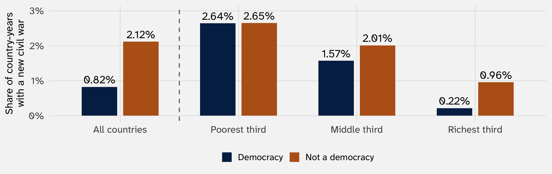
The democracy gap in civil war shrank once we compared democracies and non-democracies with similar incomes

Country-years, 1945–1999; income groups are thirds by GDP per capita. Data: Fearon and Laitin (2003), via the juanr package
That was our first look at “controlling for” something. We’ll look again today
Plus: a 10-minute break
Callback rates. Civil war rates. Divorce rates in made-up states. Every estimate so far has been a difference in means
What we really want is to compare the typical unit in each group: is the typical treated unit better or worse off than the typical untreated one?
Why should the mean be our stand-in for “typical”? Why not the mode, or the median? Why not the minimum or maximum?
Medians, modes, max, min don’t allow comparison for binary outcomes
A 0/1 outcome is the extreme case. But the question is general: what makes a number “typical”?
\[ \sum_{i=1}^{n} Y_i = Y_1 + Y_2 + \cdots + Y_n \]
Read it as: “the sum of \(Y_i\), for \(i\) from 1 to \(n\)”
The mean is that sum, divided by \(n\):
\[ \bar{Y} = \frac{1}{n} \sum_{i=1}^{n} Y_i \]
Three Senate races with 1, 2, and 6 million votes cast (made-up numbers): \(\sum Y_i = 9\), so \(\bar{Y} = 9/3 = 3\)
The ordinary mean gives every unit the same say. A weighted average gives unit \(i\) a weight \(w_i\):
\[ \bar{Y}_w = \frac{\sum_{i=1}^{n} w_i Y_i}{\sum_{i=1}^{n} w_i} \]
Three races with 1, 2, and 6 million votes, but count the third race twice (weights 1, 1, 2):
\[ \bar{Y}_w = \frac{1 \times 1 + 1 \times 2 + 2 \times 6}{1 + 1 + 2} = \frac{15}{4} = 3.75 \qquad \text{vs. the ordinary mean, } 3 \]
What happens when every \(w_i\) = 1?
A town is half under 40, half over 40. Our poll of 100 people reached 20 under 40 and 80 over 40
| Group | Share of the town | Share of the poll | Support | Weight = town share / poll share |
|---|---|---|---|---|
| Under 40 | 50% | 20% | 70% | \(0.5 / 0.2 =\) 2.5 |
| Over 40 | 50% | 80% | 40% | \(0.5 / 0.8 =\) 0.625 |
Unweighted: \(\frac{20 \times 70 + 80 \times 40}{100} =\) 46%, too close to what older people think
Weighted: \(\frac{20 \times 2.5 \times 70 + 80 \times 0.625 \times 40}{20 \times 2.5 + 80 \times 0.625} = \frac{3500 + 2000}{100} =\) 55%, the answer the whole town would give
In R: weighted.mean(support, w = weight). Every serious poll does this
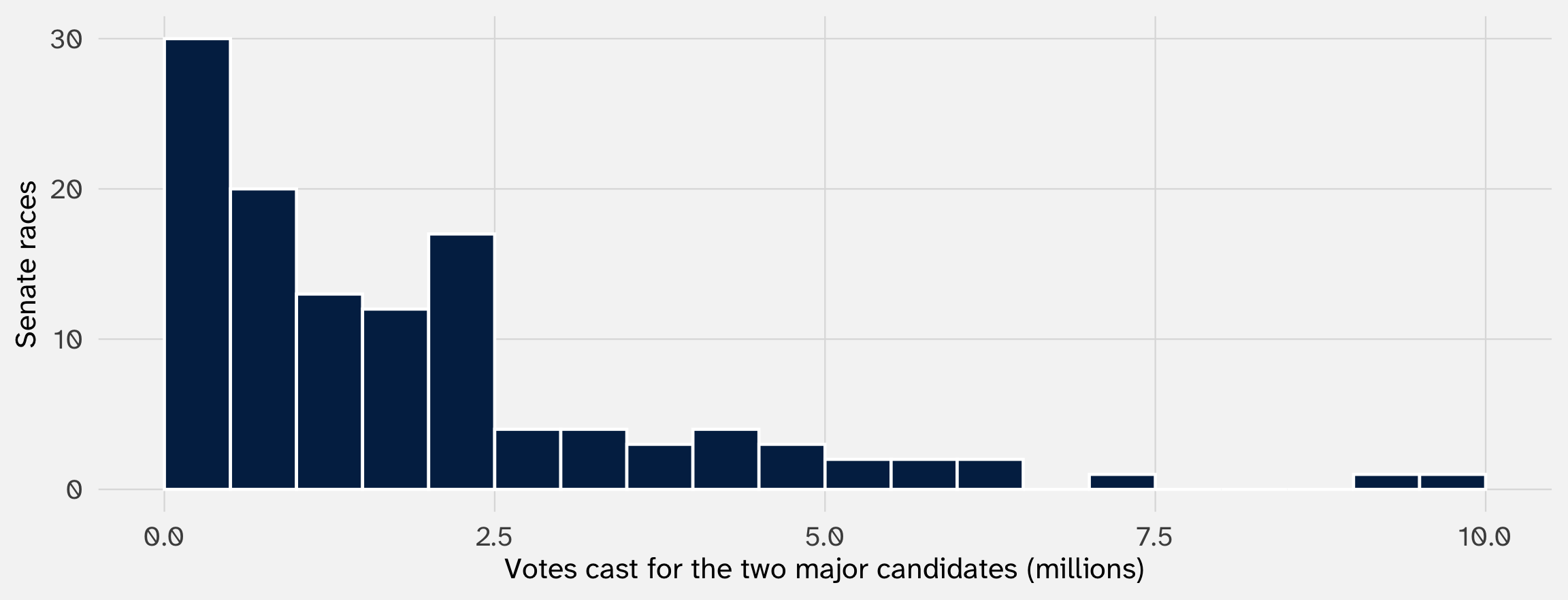
Write every race’s number of votes on a slip of paper, put the slips in a box, shake it, and draw one. What single number is your best guess for the slip you’ll draw? (Gailmard 2014)
Call your guess \(g\). Whatever you pick, you’ll usually be off. For slip \(i\), the miss is \(Y_i - g\)
Which guess counts as “best” depends on how we summarize misses
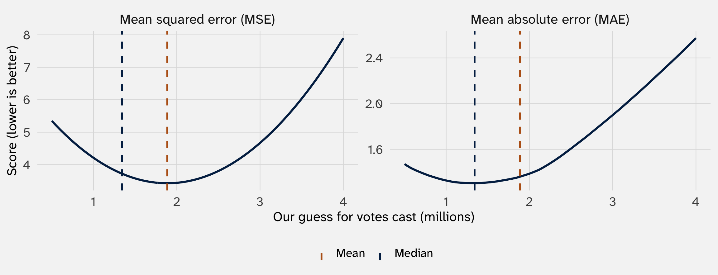
If we score each miss by its square, \((Y_i - g)^2\), the guess with the smallest average miss turns out to be the mean of Y → \(\bar{Y}\)
Let’s see why →
Back to three races with 1, 2, and 6 million votes. Say we guess 4 million for whichever slip we draw
| Race | Votes cast, \(Y_i\) | Guess, \(g\) | Miss, \(Y_i - g\) |
|---|---|---|---|
| A | 1 | 4 | \(-3\) |
| B | 2 | 4 | \(-2\) |
| C | 6 | 4 | \(+2\) |
We want one number that says how bad this guess is overall. What should it be?
| Guess \(g\) | Votes cast, \(Y_i\) | Misses, \(Y_i - g\) | Sum of the misses | Squared misses | Sum of the squares |
|---|---|---|---|---|---|
| 4 | \(1, 2, 6\) | \(-3, -2, +2\) | \(-3\) | \(9, 4, 4\) | 17 |
| 3 | \(1, 2, 6\) | \(-2, -1, +3\) | \(0\) | \(4, 1, 9\) | 14 |
Adding raw misses fails: a guess of 3 misses every race, yet its misses sum to zero
Squaring fixes it: squares are never negative, so misses can’t cancel (what’s an alternative to squaring?)
We score guesses using the mean squared error (MSE)
\[ \text{MSE}(g) = \frac{1}{n} \sum_{i=1}^{n} (Y_i - g)^2 \]
| Step | Piece | Read it as |
|---|---|---|
| 1 | \(Y_i - g\) | How far the guess misses slip \(i\) |
| 2 | \((\ldots)^2\) | Square that miss |
| 3 | \(\sum_{i=1}^{n}\) | Add up the squared misses for all \(n\) slips |
| 4 | \(\frac{1}{n}\) | Divide by \(n\): the average squared miss |
it’s a sum of \(n\) things divided by \(n\), a mean, so the name says exactly what it is
| Guess \(g\) | MSE(\(g\)) |
|---|---|
| 0 | 13.67 |
| 1 | 8.67 |
| 2 | 5.67 |
| 3 | 4.67 |
| 4 | 5.67 |
| 5 | 8.67 |
| 6 | 13.67 |
| 7 | 20.67 |
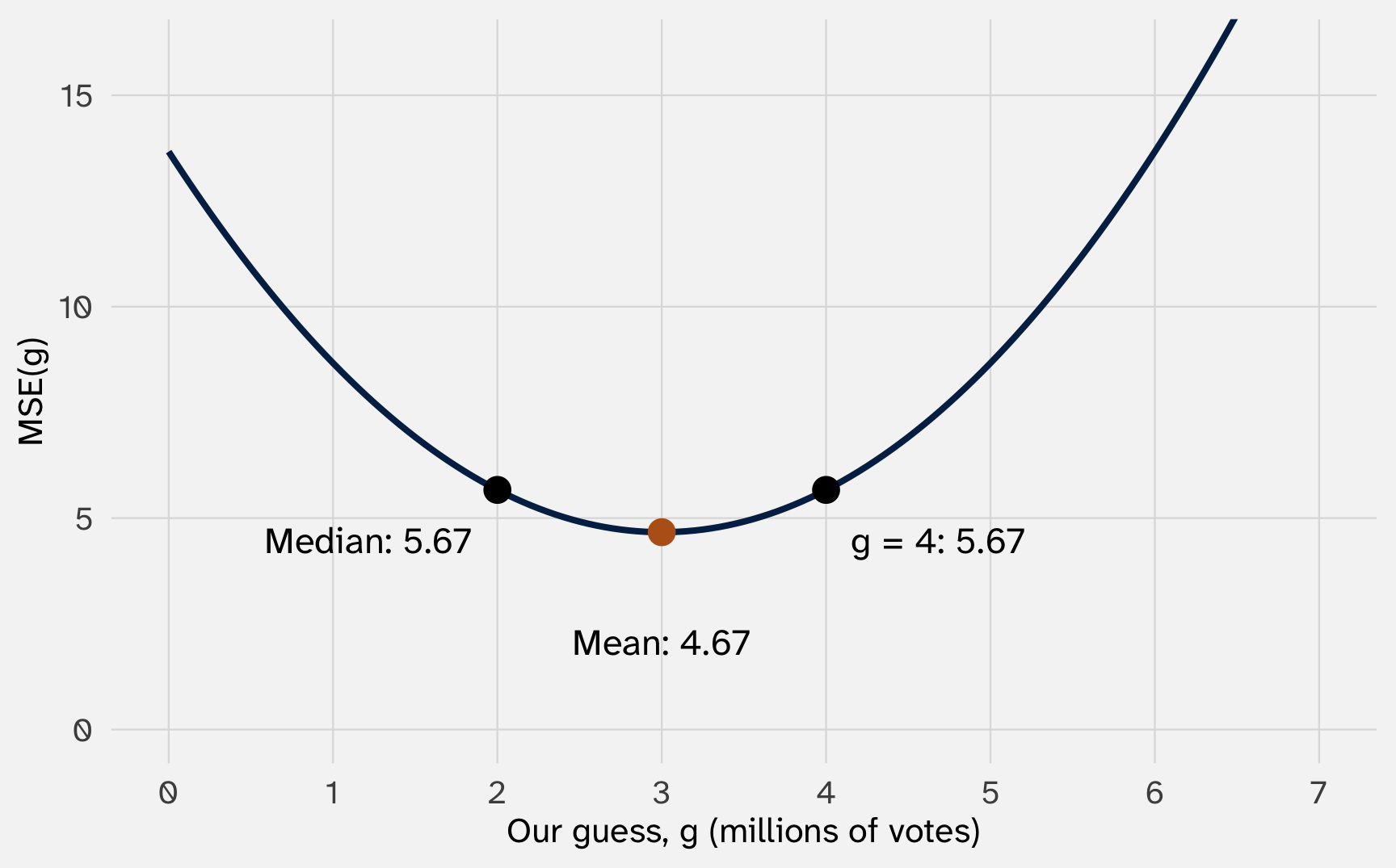
The curve is a bowl with one bottom, at 3: the mean. Every other guess does worse
Might feel like over-kill for motivating the average, but MSE shows up everywhere:
| Where | The curve | We look for its… |
|---|---|---|
| Today | MSE of a single guess | Bottom: the mean |
| Later today | MSE of every possible straight line | Bottom: the regression line (“least squares”) |
| Week 8 | An estimator’s MSE = bias2 + variance | Bottom: the best tradeoff between bias and noise |
| POL 212 | MSE of lines with many variables | Bottom, found with calculus and matrices |
| POL 213 | The likelihood of the data | Top: maximum likelihood |
| Machine learning | Prediction error | Bottom, by walking downhill step by step |
\[ \sum_{i=1}^{n} (Y_i - \bar{Y}) = 0 \]
For 1, 2, and 6, the misses from the mean (3) are \(-2\), \(-1\), and \(+3\). They add up to zero
So what?
The mean is the balance point of the data: misses above it exactly cancel misses below it
\[ \text{If } X_i = k \times Y_i \text{ for every unit, then } \bar{X} = k \times \bar{Y} \]
# A tibble: 2 × 4
race as_share as_percent_k_y as_percent_k_ybar
<chr> <dbl> <dbl> <dbl>
1 black 0.0645 6.45 6.45
2 white 0.0965 9.65 9.65
So what?
Units follow the data. The résumé gap is 0.032 as a share or 3.2 as percentage points: the same finding. Dollars to euros, shares to percents, thousands to millions: means (and differences in means) rescale by the same factor
\[ \text{If } X_i = Y_i + k \text{ for every unit, then } \bar{X} = \bar{Y} + k \]
Why: adding \(k\) to all \(n\) values adds \(n \times k\) to the sum; dividing by \(n\) leaves \(k\)
# A tibble: 2 × 4
oil polity polity_0_to_20_ky polity_0_to_20_ky_bar
<dbl> <dbl> <dbl> <dbl>
1 0 0.188 10.2 10.2
2 1 -3.87 6.13 6.13
So what?
Shifting a scale moves every average, but the gap between groups doesn’t budge: the \(+k\) cancels in the subtraction. Lets you scale variables to make them more interpretable
We squared to stop misses from canceling. Another way is the absolute value, \(\lvert Y_i - g \rvert\): every miss counts by its size
\[ \text{MAE}(g) = \frac{1}{n} \sum_{i=1}^{n} \lvert Y_i - g \rvert \qquad \text{(mean absolute error)} \]
It turns out that the winner on MAE is not the mean, but the median
Let’s look at some real data to test this out
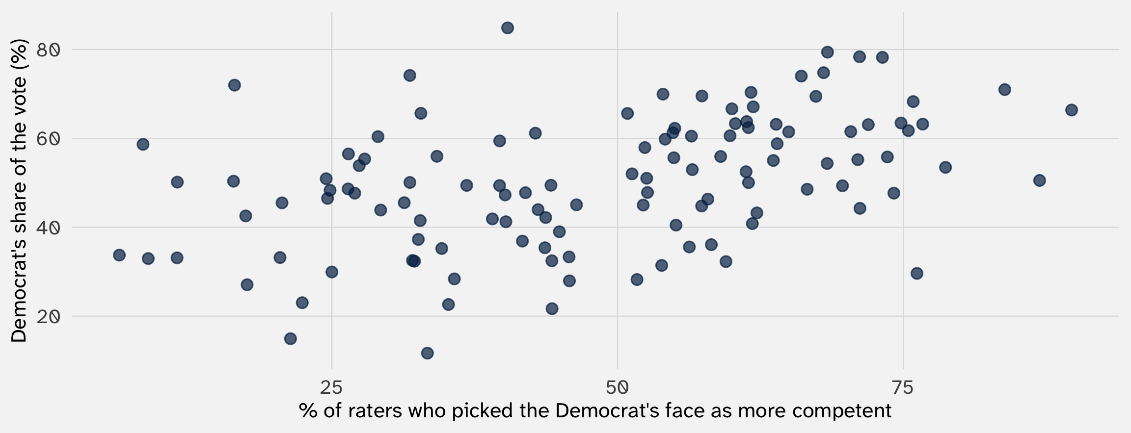
Todorov et al. (2005) showed people the faces of two Senate candidates for one second and asked: who looks more competent?
| Year | State | Winner | Loser | % picking the Democrat’s face | Democrat’s % of the vote |
|---|---|---|---|---|---|
| 2000 | CA | Feinstein | Campbell | 56 | 60.5 |
| 2000 | DE | Carper | Roth | 34 | 56.0 |
| 2000 | FL | Nelson | McCollum | 61 | 52.5 |
| 2000 | GA | Miller | Mattingly | 54 | 59.8 |
| 2000 | HI | Akaka | Carroll | 68 | 74.8 |
| 2000 | IN | Lugar | Johnson | 32 | 32.5 |
The candidate whose face looked more competent won 72% of these races

Download face.csv into your data/ folder
total_votes
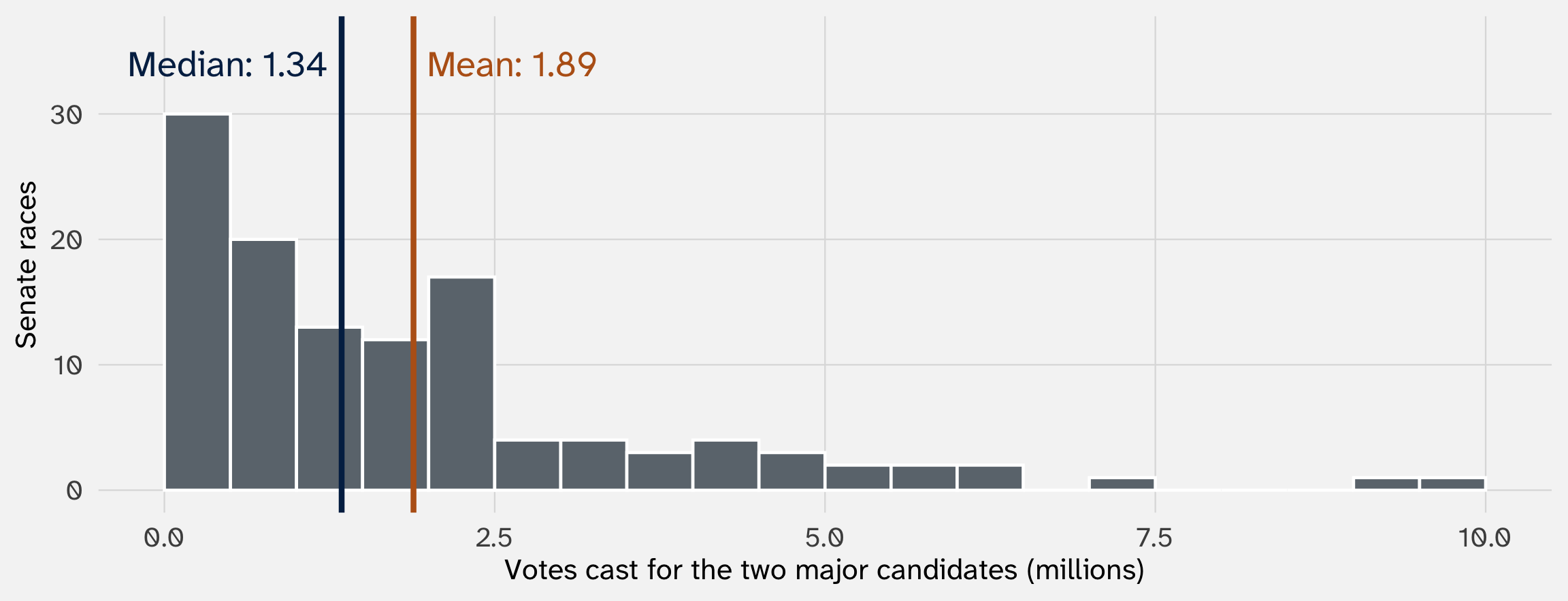
The mean (1.89 million) has the smallest MSE. The median (1.34 million) has the smallest MAE
Squaring means that all errors don’t count the same: large errors become especially “important”
Three races (1, 2, and 6 million votes: mean 3, median 2). Add a fourth. What happens to the mean and the median?
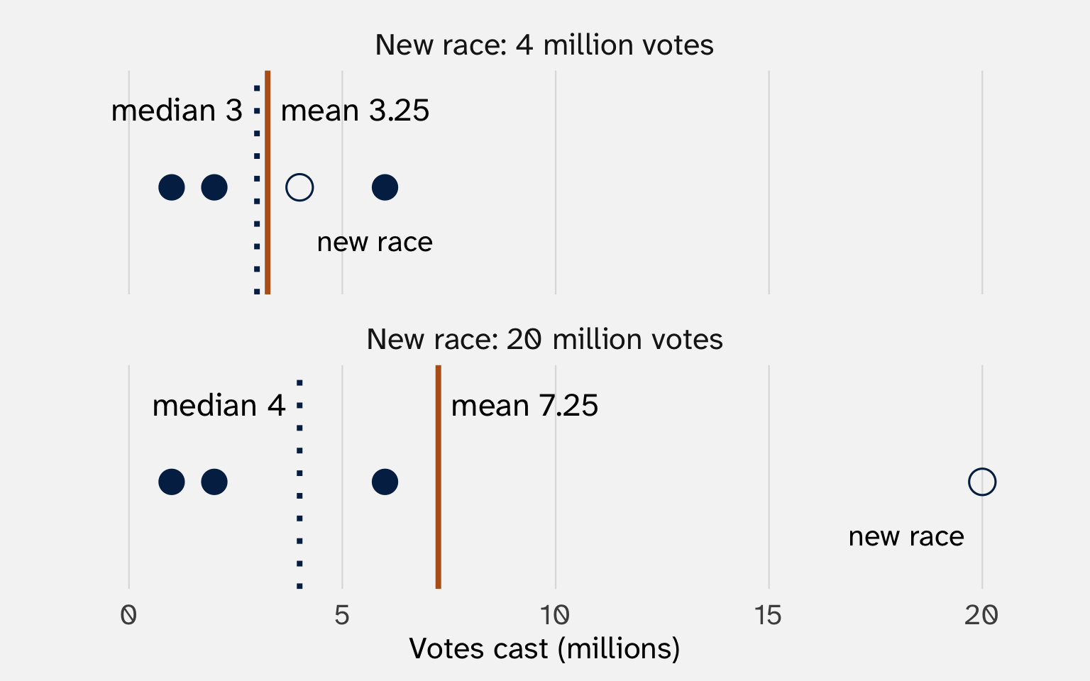
| Miss | Absolute (MAE) | Squared (MSE) |
|---|---|---|
| 1 | 1 | 1 |
| 2 | 2 | 4 |
| 4 | 4 | 16 |
| 17 | 17 | 289 |

Squaring makes big misses count a lot, so the mean chases California and Texas. The median doesn’t care how big they are
Week 1: the average of the differences equals the difference of the averages. That’s what let us learn an average effect from two groups
| Bike | Bus | Bus \(-\) bike | |
|---|---|---|---|
| You | 10 | 20 | 10 |
| Your roommate | 15 | 15 | 0 |
| Your friend | 20 | 40 | 20 |
| Average | 15 | 25 | 10 |
| Median | 15 | 20 | 10 |
Difference of the averages: \(25 - 15 = 10\) ✓
Difference of the medians: \(20 - 15 = 5\), but the median of the differences is 10 ✗
| Use the mean when you want to… | Use the median when you want to… |
|---|---|
| Estimate an effect. Only averages combine: the difference of the means is the mean of the differences | Describe a typical unit in skewed data: income, wealth, house prices, campaign money |
| Measure uncertainty. One smooth bottom to find; the central limit theorem gives its standard error (week 7) | Resist outliers and data errors. A few wild values barely move it |
| Add things up. Mean × \(n\) = the total: votes, spending, deaths | Study the middle of a distribution, not its average (median regression) |
When the two disagree, report both: the gap tells you about skew. Running for Congress, the median candidate raised $15k; the mean, $641k. Data: Bonica (2014), via the juanr package

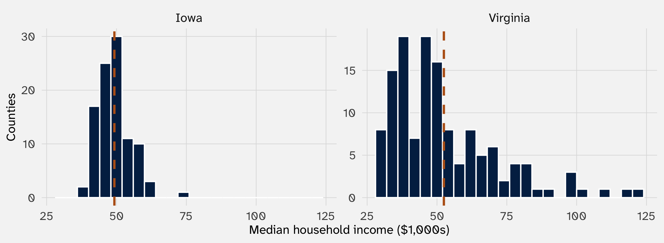
Median household income, 2009–2013, in 99 Iowa counties and 134 Virginia counties and independent cities. Dashed lines: each state’s average. Data: US Census Bureau, via the socviz package
The averages are close: $49k and $52k. But Iowa’s counties huddle around theirs, while Virginia’s run from $28k to $122k
| County | Income | State average | Distance, \(Y_i - \bar{Y}\) |
|---|---|---|---|
| Martinsville city | $28k | $52k | -24k |
| Surry County | $47k | $52k | -5k |
| Loudoun County | $122k | $52k | +70k |
How far is each county from the average county in its state?
Average the distances? They always add up to zero (property 1 of means): the counties above cancel the ones below
So we do what we did for the MSE: square the distances, then average them
\[ \text{Var}(Y) = \frac{1}{n} \sum_{i=1}^{n} (Y_i - \bar{Y})^2 \]
| Step | Piece | Read it as |
|---|---|---|
| 1 | \(Y_i - \bar{Y}\) | How far county \(i\) sits from the average |
| 2 | \((\ldots)^2\) | Square that distance |
| 3 | \(\sum_{i=1}^{n}\), \(\frac{1}{n}\) | Add them up and divide by \(n\): the average squared distance |
Iowa: 35. Virginia: 367. In thousands of dollars, squared. What’s a squared dollar?
\[ \text{SD}(Y) = \sqrt{\text{Var}(Y)} \]
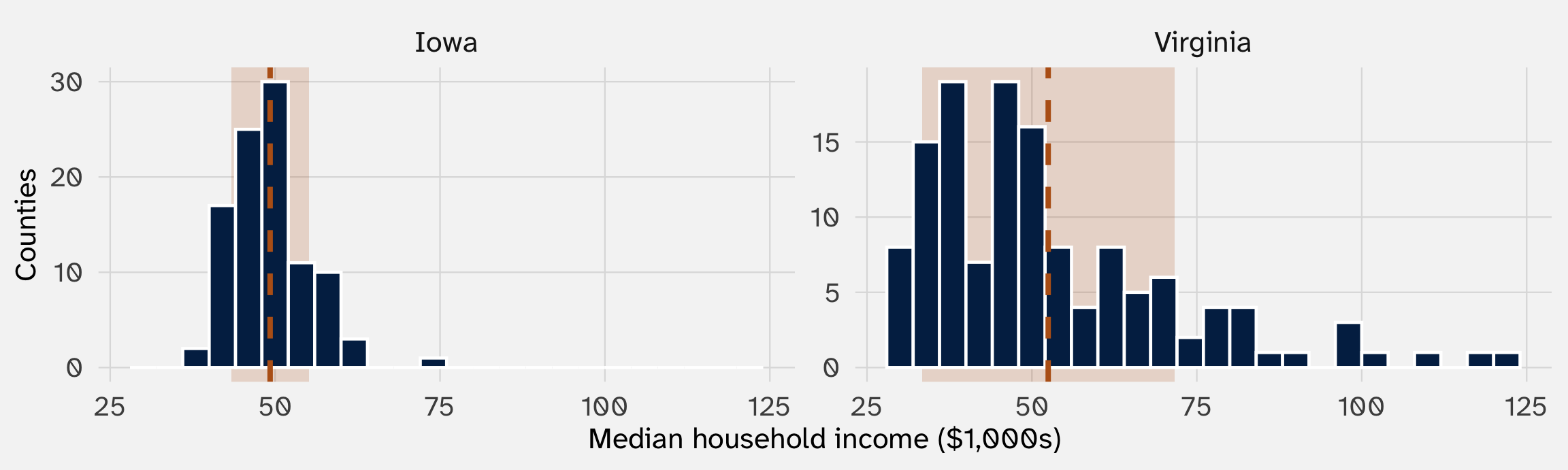
Shaded: one standard deviation on either side of each state’s average. Data: US Census Bureau, via the socviz package
A typical Iowa county sits about $5.9k from its state’s average; a typical Virginia county, about $19.1k
mutate() to find each race’s miss from the mean, then square itsummarize() to average the squared misses (the variance), then take the square root with sqrt()sd(d_share). It should be the same number.sd() divides by n – 1, not n# A tibble: 1 × 2
sd_by_hand sd_r
<dbl> <dbl>
1 14.7 14.7
With 119 races, the two barely differ. Why \(n - 1\)? Later in the course, we’ll see that \(n-1\) is necessary when we’re talking about a sample from a population
Compare the two formulas:
\[ \text{MSE}(g) = \frac{1}{n} \sum_{i=1}^{n} (Y_i - g)^2 \qquad\qquad \text{Var}(Y) = \frac{1}{n} \sum_{i=1}^{n} (Y_i - \bar{Y})^2 \]
The variance is the MSE with the mean plugged in as the guess: \(\text{Var}(Y) = \text{MSE}(\bar{Y})\)
So the variance is the height of the bottom of the MSE curve. For 1, 2, and 6, the curve bottomed out at 4.67: that’s their variance
Spread isn’t a separate idea from the center: it’s how well the center does as a guess
Week 1’s standard error is built from each group’s variance and size:
\[ SE = \sqrt{\frac{\text{Var}_{\text{AA}}}{n_{\text{AA}}} + \frac{\text{Var}_{\text{W}}}{n_{\text{W}}}} \]
\[ SE = \sqrt{\frac{0.0603}{2435} + \frac{0.0872}{2435}} = \mathbf{0.0078} \]
| Callback (1) | |
|---|---|
| African American-sounding name | -0.032 |
| (0.0078) | |
| Intercept | 0.097 |
| (0.0055) | |
| Résumés | 4,870 |
Linear regression. Outcome: callback = 1 if the employer called back, 0 if not. Standard errors in parentheses.
The same number: the table’s standard error is this formula
We’ll see why we use this formula to quantify uncertainty later in the course
When would we want to compare standard deviations?
| Concept | It’s the spread of… |
|---|---|
| Political polarization | Legislators’ ideology |
| Inequality | Income or wealth |
| Ruggedness of terrain | Elevation |
| Electoral volatility | Parties’ vote shares from one election to the next |
For each, the mean misses the point: two countries with the same average income can have very different inequality

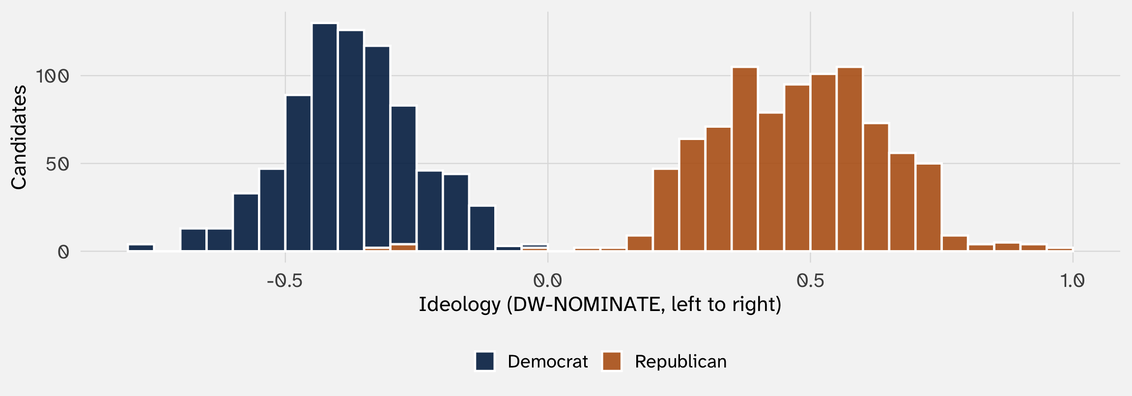
Members of Congress running in 2012, 2016, and 2018, by party. Data: Bonica (2014), via the juanr package
SD of ideology in all of Congress: 0.45. Within the Democrats: 0.13. Within the Republicans: 0.17

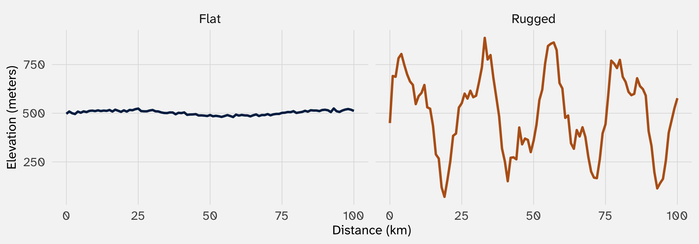
Two made-up regions with the same average elevation, about 501 meters. Simulated data
Same mean; SDs of 11 and 206 meters. Carter, Shaver, and Wright (2019) argue rugged land kept ethnic groups apart, and that this is part of why rugged countries have more civil war
Richer countries tend to be democracies
Older people are more likely to vote
Civil wars tend to break out in poor countries
None of these says every rich country is a democracy, or that being rich causes democracy. Each one says two things tend to go together
“The correlation between two features of the world is the extent to which they tend to occur together.”
— Bueno de Mesquita and Fowler (2021, 13)
| When one feature occurs, the other… | The two are… | Example |
|---|---|---|
| tends to occur too | positively correlated | A country’s income and being a democracy |
| is no more or less likely | uncorrelated | A country’s income and the first letter of its name |
| tends not to occur | negatively correlated | A country’s income and a civil war breaking out |
Two questions to ask of any correlation: which direction, and how strong?

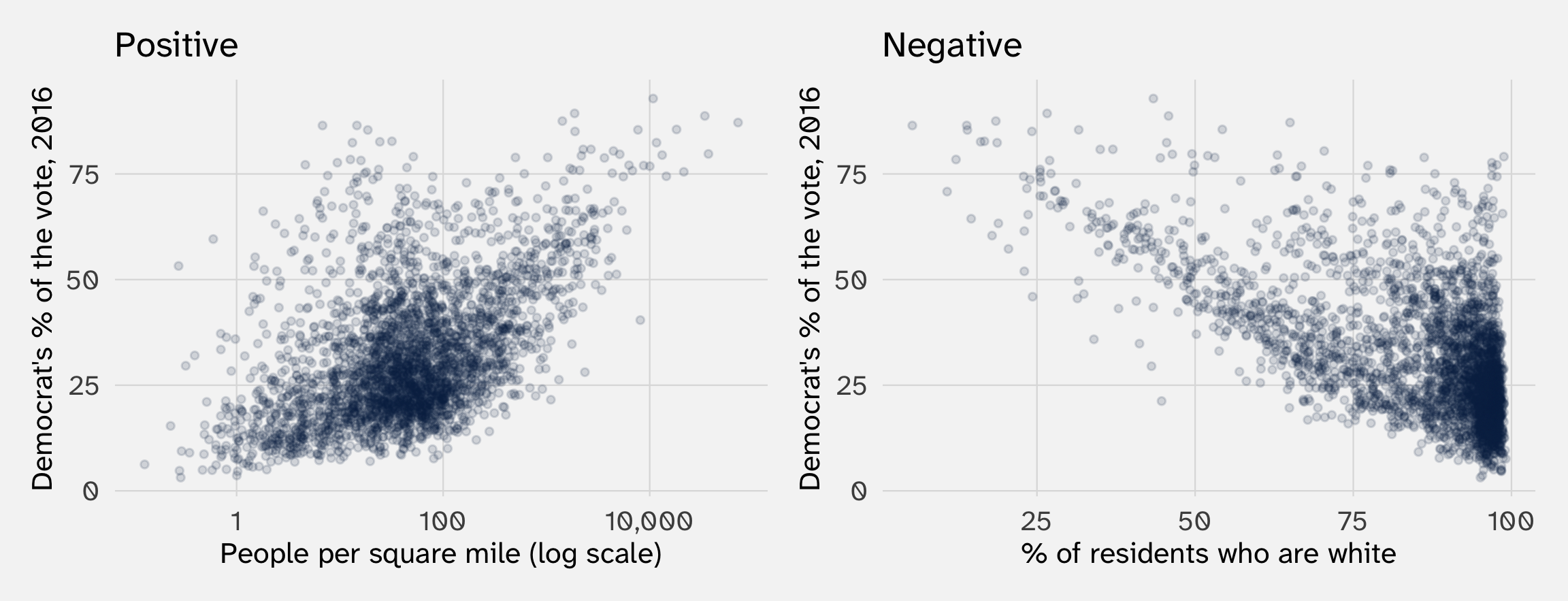
Each dot is one of 3,112 US counties. Data: US Census Bureau and county election returns, via the socviz package
Denser counties voted more Democratic in 2016; whiter counties voted less Democratic

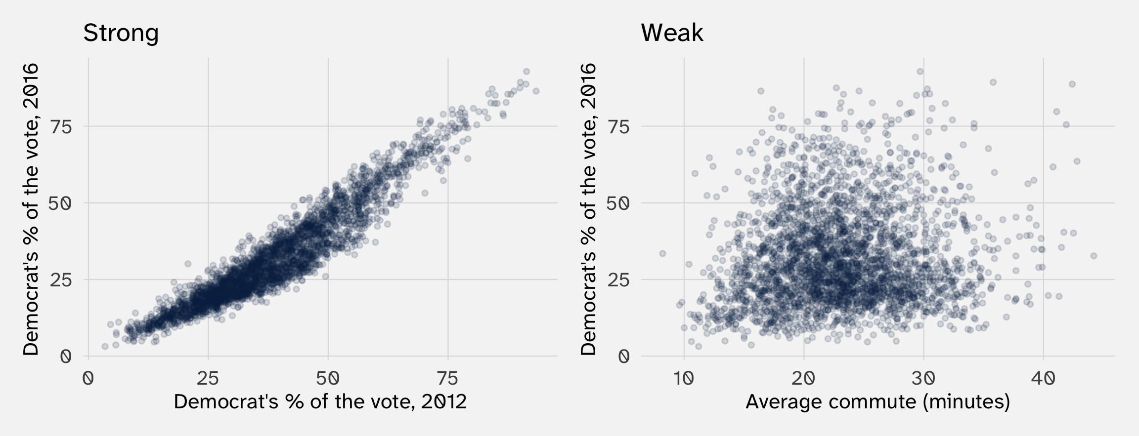
Each dot is one of 3,112 US counties. Data: US Census Bureau and county election returns, via the socviz package
Know a county’s 2012 vote and you can guess its 2016 vote closely. Know its commute, and your guess barely improves
Knowing whose face looked more competent changes our guess about who won. That’s what it means for two variables to be related
We write the average of \(Y\) among units with a given value of \(X\) as
\[ E[Y \mid X = x] \]
“The expected value of \(Y\), given that \(X\) equals \(x\)”: the conditional mean

Direction: positive. Strength: somewhere in between. With no groups to compare, how do we put one number on it?

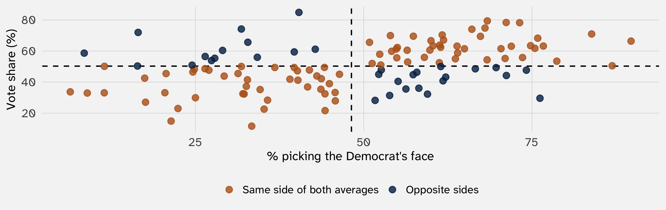
87 of 119 races sit on the same side of both averages: above on both, or below on both. That’s “tend to occur together”
But counting treats a race just past the average like one far out. Covariance weighs each race by how far it sits from both averages
\[ \text{Cov}(X, Y) = \frac{1}{n} \sum_{i=1}^{n} (X_i - \bar{X})(Y_i - \bar{Y}) \]
| Step | Piece | Read it as |
|---|---|---|
| 1 | \(X_i - \bar{X}\) and \(Y_i - \bar{Y}\) | How far unit \(i\) sits from average on \(X\), and on \(Y\) |
| 2 | \((\ldots)(\ldots)\) | Multiply the two misses |
| 3 | \(\sum_{i=1}^{n}\) | Add up the products for all \(n\) units |
| 4 | \(\frac{1}{n}\) | Divide by \(n\): the average product |
Same recipe as the variance, except we multiply two different misses instead of squaring one
| Race | X | X − X̄ | Y | Y − Ȳ | Product |
|---|---|---|---|---|---|
| HI 2004 | 73 | +25 | 78 | +28 | |
| NM 2000 | 75 | +27 | 62 | +11 | |
| WY 2000 | 22 | -26 | 23 | -27 | |
| IN 2000 | 32 | -16 | 33 | -18 | |
| IL 2004 | 16 | -32 | 72 | +22 | |
| UT 2004 | 76 | +28 | 30 | -21 |
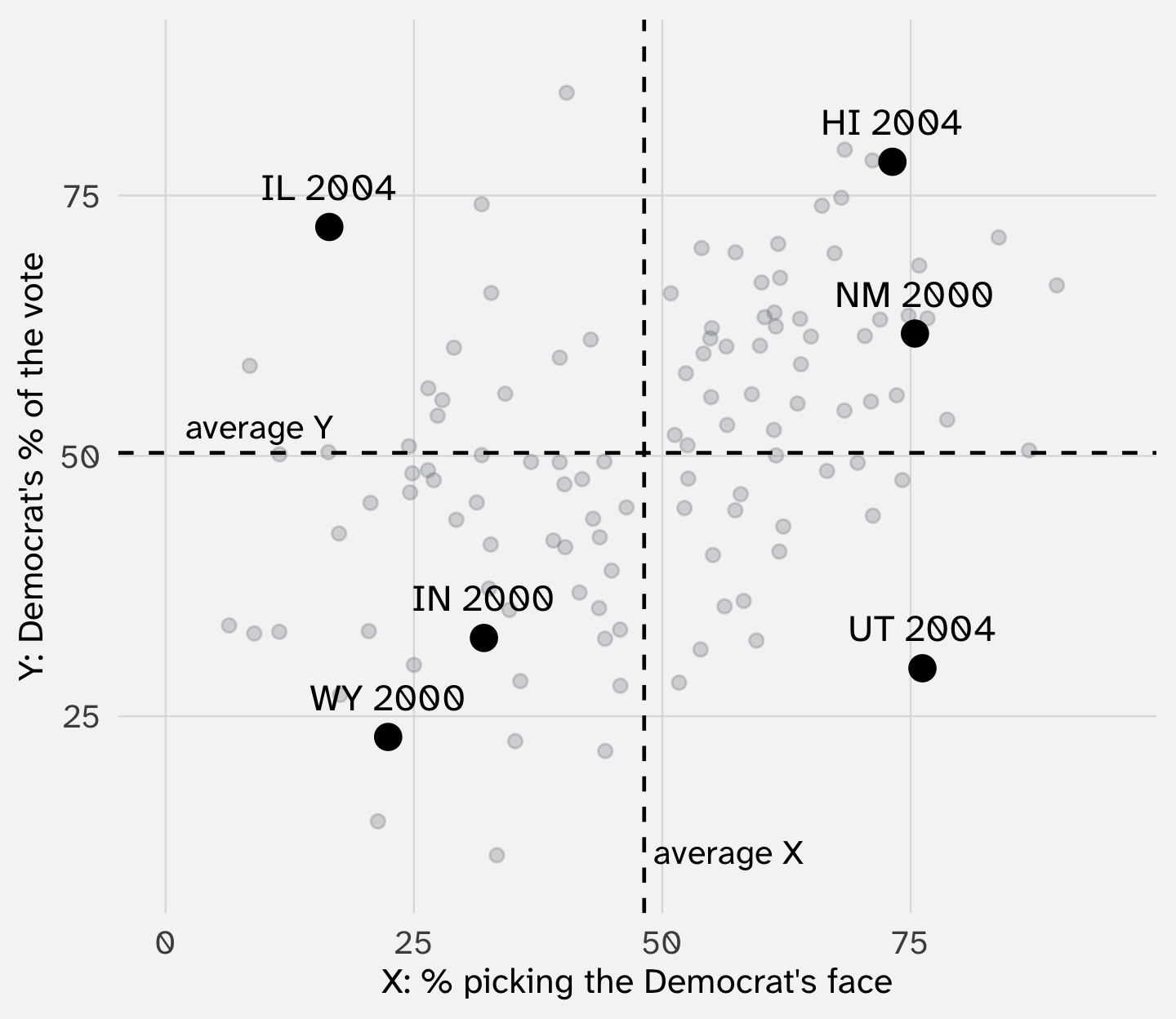
The dashed lines are the averages. They split the plot into four corners
| Race | X | X − X̄ | Y | Y − Ȳ | Product |
|---|---|---|---|---|---|
| HI 2004 | 73 | +25 | 78 | +28 | +698 |
| NM 2000 | 75 | +27 | 62 | +11 | |
| WY 2000 | 22 | -26 | 23 | -27 | |
| IN 2000 | 32 | -16 | 33 | -18 | |
| IL 2004 | 16 | -32 | 72 | +22 | |
| UT 2004 | 76 | +28 | 30 | -21 |
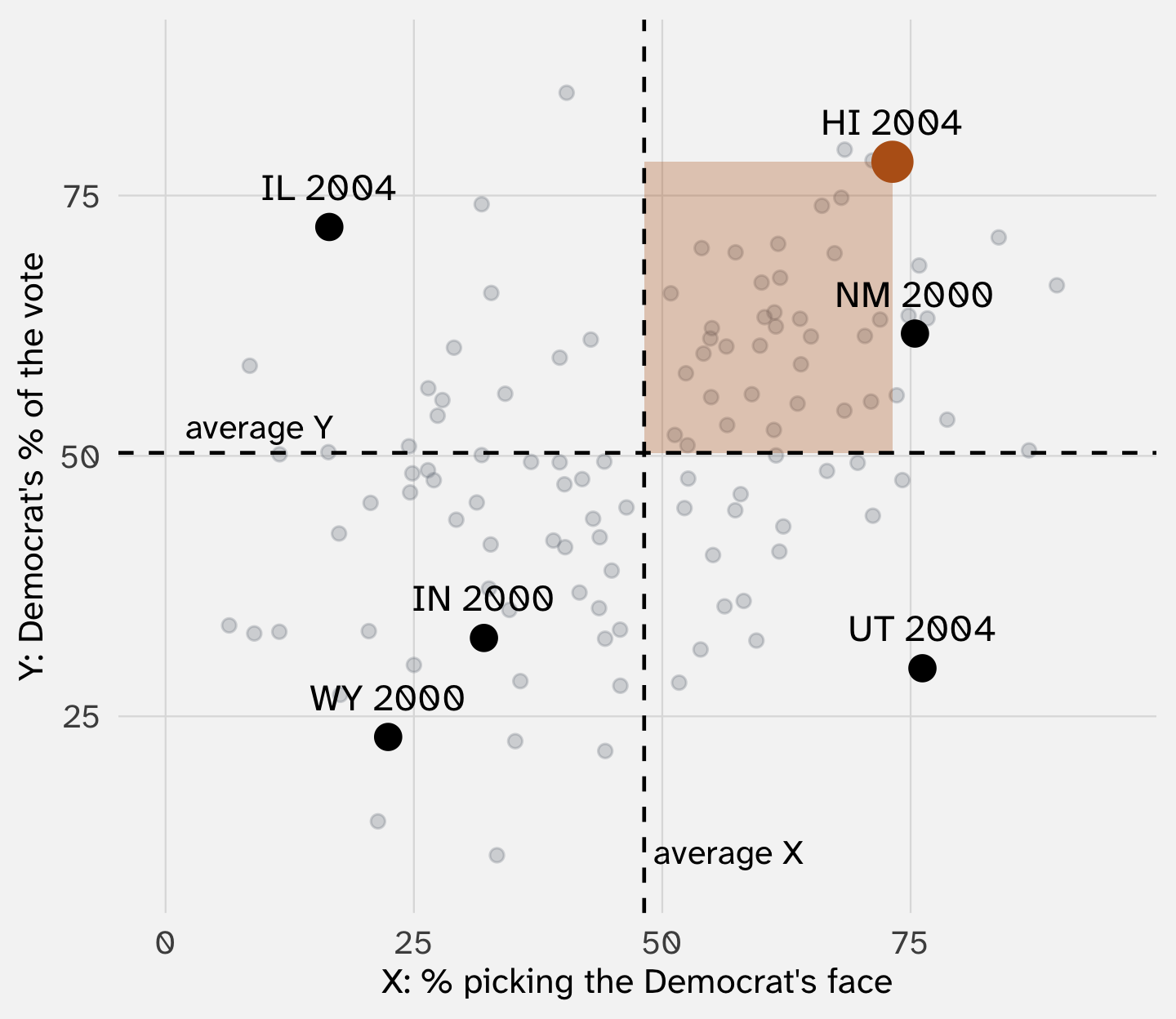
Hawaii 2004: 25 points above average on looks, 28 above on votes. 25 × 28 ≈ +698: it pushes the covariance up
| Race | X | X − X̄ | Y | Y − Ȳ | Product |
|---|---|---|---|---|---|
| HI 2004 | 73 | +25 | 78 | +28 | +698 |
| NM 2000 | 75 | +27 | 62 | +11 | |
| WY 2000 | 22 | -26 | 23 | -27 | +703 |
| IN 2000 | 32 | -16 | 33 | -18 | |
| IL 2004 | 16 | -32 | 72 | +22 | |
| UT 2004 | 76 | +28 | 30 | -21 |
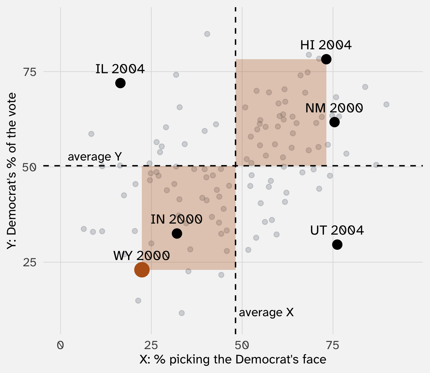
Wyoming 2000: -26 on looks, -27 on votes. Two negatives make a positive: +703. Low with low also pushes the covariance up
| Race | X | X − X̄ | Y | Y − Ȳ | Product |
|---|---|---|---|---|---|
| HI 2004 | 73 | +25 | 78 | +28 | +698 |
| NM 2000 | 75 | +27 | 62 | +11 | |
| WY 2000 | 22 | -26 | 23 | -27 | +703 |
| IN 2000 | 32 | -16 | 33 | -18 | |
| IL 2004 | 16 | -32 | 72 | +22 | -687 |
| UT 2004 | 76 | +28 | 30 | -21 |
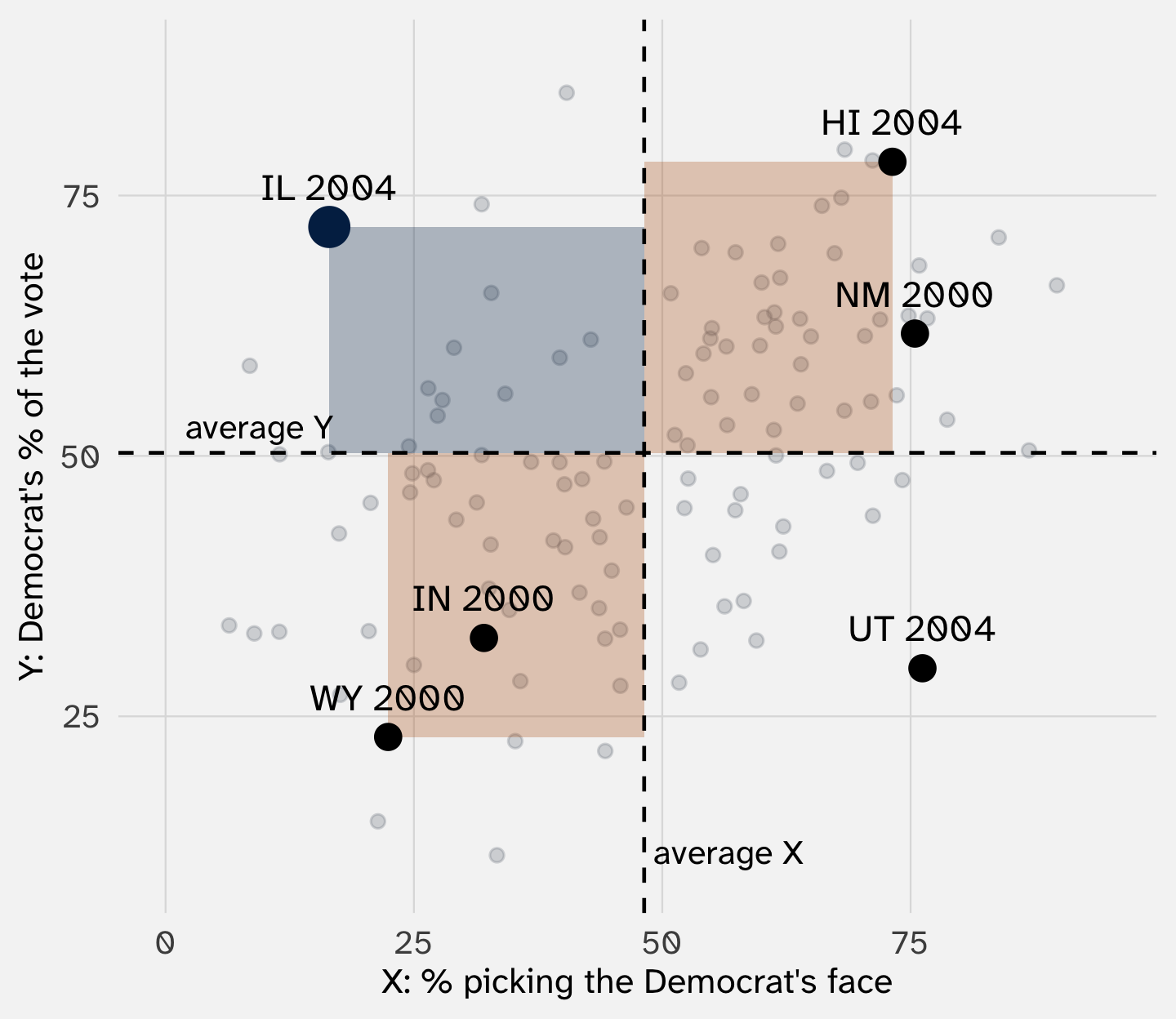
Illinois 2004: -32 on looks, +22 on votes: -687. A race that bucks the pattern pulls the covariance down
| Race | X | X − X̄ | Y | Y − Ȳ | Product |
|---|---|---|---|---|---|
| HI 2004 | 73 | +25 | 78 | +28 | +698 |
| NM 2000 | 75 | +27 | 62 | +11 | +312 |
| WY 2000 | 22 | -26 | 23 | -27 | +703 |
| IN 2000 | 32 | -16 | 33 | -18 | +287 |
| IL 2004 | 16 | -32 | 72 | +22 | -687 |
| UT 2004 | 76 | +28 | 30 | -21 | -579 |
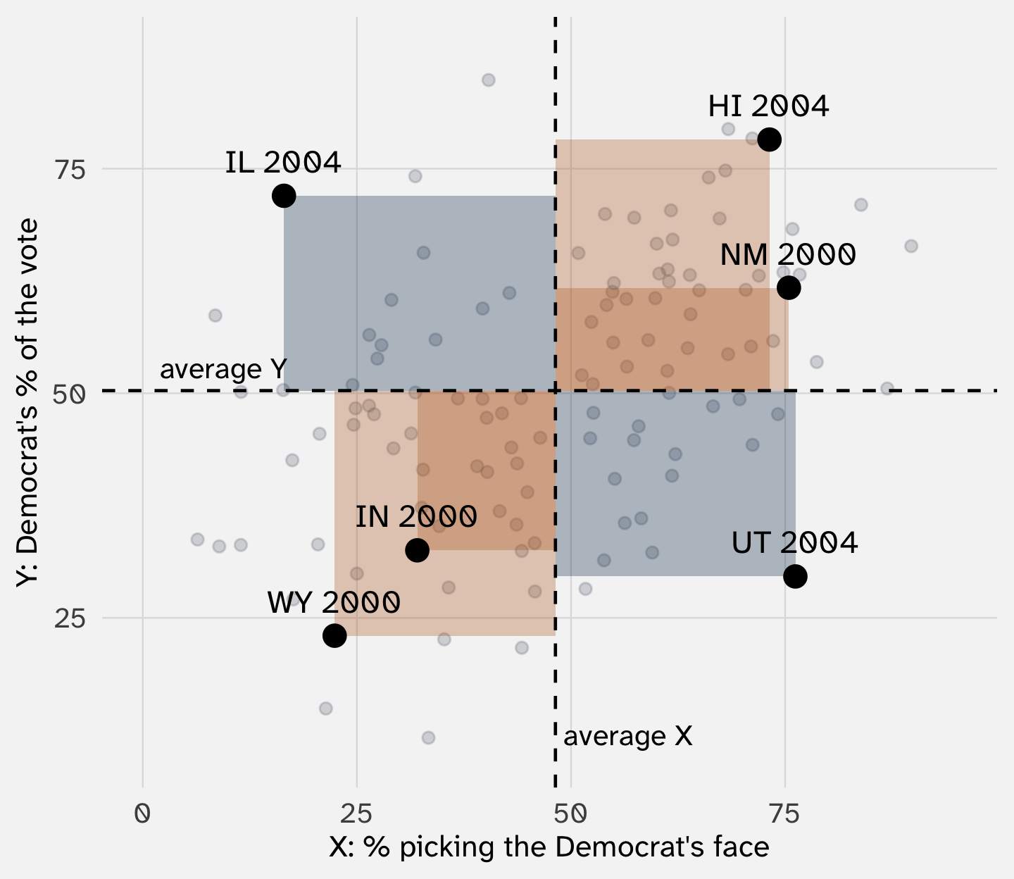
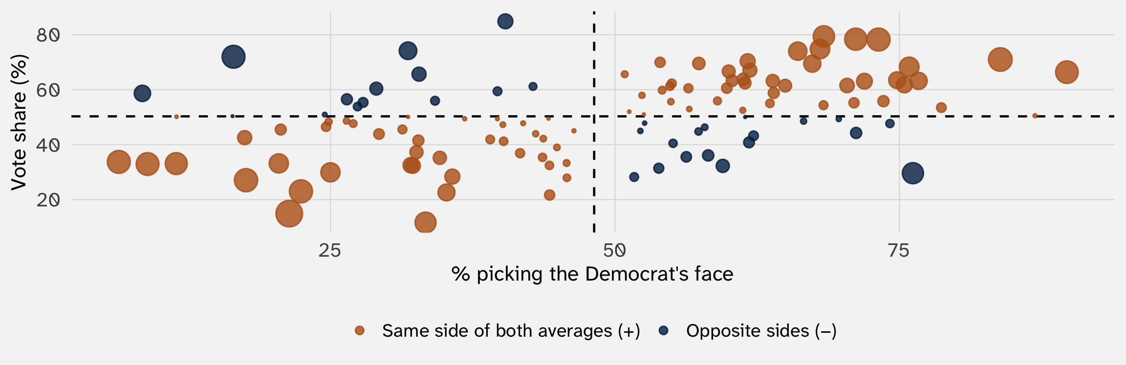
Orange rectangles add, blue ones subtract. These six sum to 734; divided by 6, that’s about 122

Big dots sit far from both averages, so they count the most. The orange corners still outweigh the blue: the covariance is positive (121.8)
The covariance here is 121.8, in “percent of raters times percentage points of the vote.” Is that big?
Divide by both standard deviations and the units cancel:
\[ r = \frac{\text{Cov}(X, Y)}{\text{SD}(X) \, \text{SD}(Y)} \]
The correlation runs from \(-1\) (a perfect line sloping down) to \(+1\) (a perfect line sloping up)
For faces and votes: r = 0.43

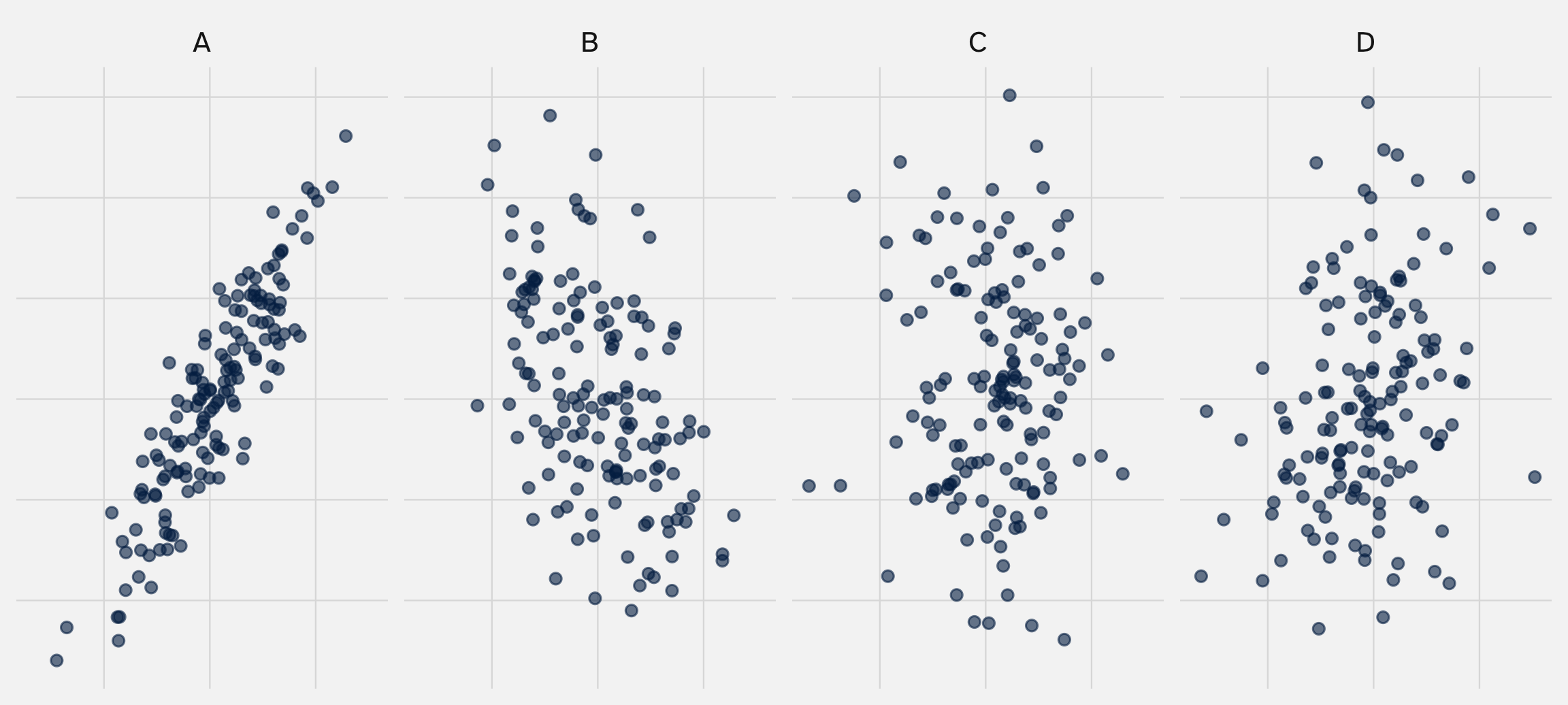
Write down a guess for each panel
| Panel | Correlation in this sample |
|---|---|
| A | 0.90 |
| B | -0.48 |
| C | 0.01 |
| D | 0.29 |
The correlation, 0.43, says faces and votes move together, and how tightly. It doesn’t say how much
If 10 more points of raters picked a candidate’s face, how much more of the vote would they get? The correlation can’t say: it has no units
But “how much” is what most applications need. With two groups, we compared two averages. Competence ratings take many values
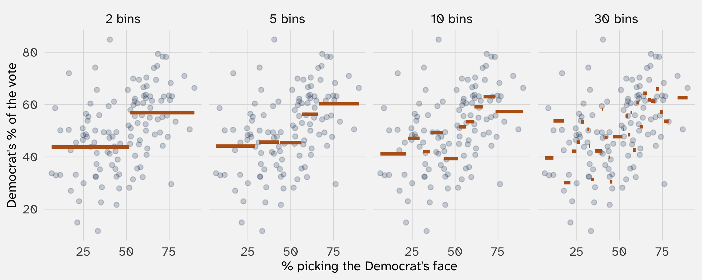
The natural move: chop \(X\) into bins and take the average of \(Y\) in each bin
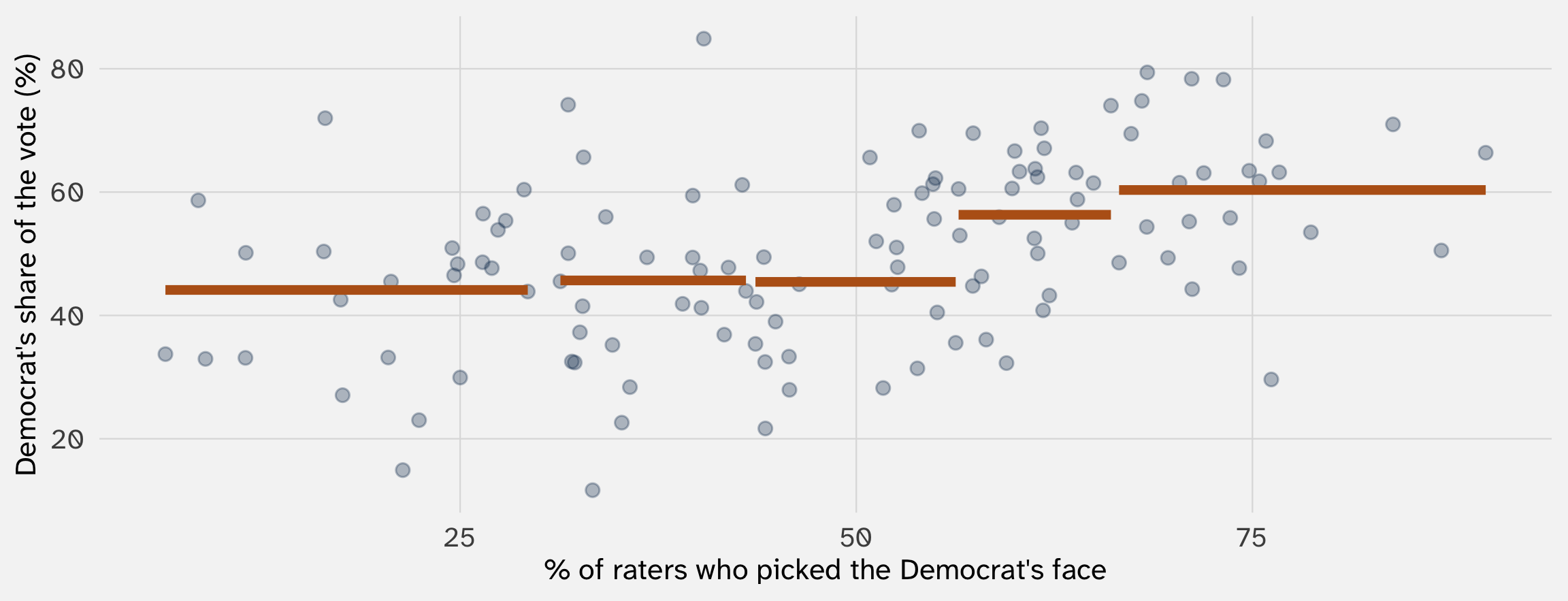
That’s a conditional mean, \(E[Y \mid X]\), one bin at a time

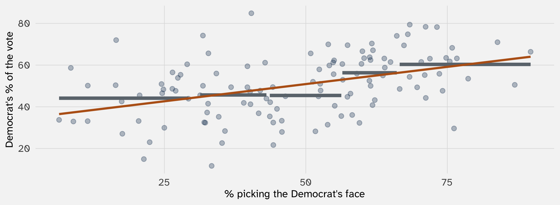
Orange lines: the average vote share among races in each fifth of competence ratings. Data: Todorov et al. (2005), via Imai and Williams (2022)
We could then compare \(E[Y \mid X = 1]\) vs \(E[Y \mid X = 2]\)

With 30 bins, each average rests on about 4 races. They’re very noisy
A rerun or more data of these elections would give a very different set of bins
Where we have no data, bins tell us nothing
And the cutoffs are arbitrary: move one, and the picture changes
Instead of fixed bins, average the races near each value of \(X\), then slide over and do it again
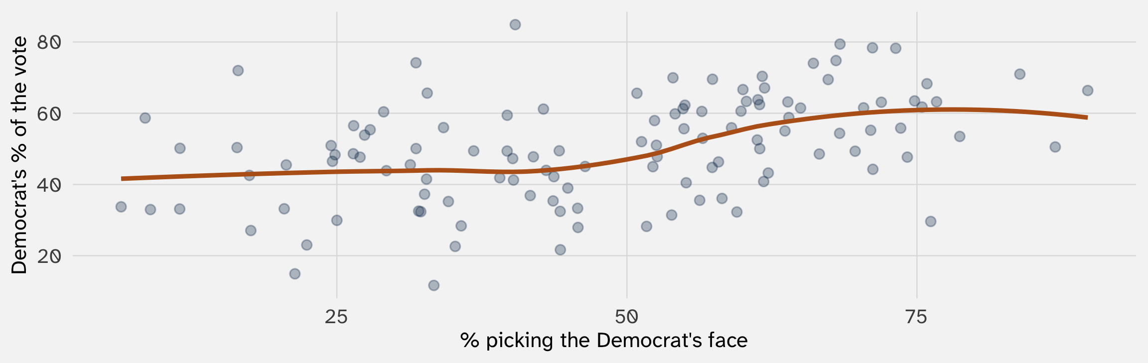
That’s what geom_smooth() draws if you don’t give it a method (a “LOESS” curve). Smoother, but still hard to sum up in one number

Forcing a shape (the line) fills in the gaps and smooths out some of the noise, at the cost of missing curves
The slope of the line also characterizes the relationship in term of \(X\) and \(Y\) units
Linear regression. Outcome: the Democrat’s share of the two-party vote, in percent. Standard errors in parentheses.
Read the slope: each extra point of raters picking the Democrat’s face goes with 0.33 points more of the vote
So a race where 70% of raters picked the Democrat’s face, vs. one where 30% did, goes with about 13.2 points more of the vote for the Democrat

Incumbents are older, more polished, and better known. They may look more competent, and they win more votes for many other reasons
Same question as last week: what if the relationship is all a third variable, \(Z\)?
| Tool | Distances from… |
|---|---|
| Mean squared error | A guess |
| Variance and SD | The mean |
| Covariance and correlation | The mean of \(X\) and the mean of \(Y\) |
| A regression line | The line’s prediction (the conditional mean) |
Exam 1 covers weeks 1–3 and takes the first half of class
Then we start probability: if we ran the world again, would we get the same answer?
POL 211 · Fall 2026