POL 211 · Week 2
University of California, Davis
October 6, 2026
Systematic part: the patterns our theories are about, like how much a name changes an employer’s chance of calling back
Random part: everything else, like which manager opened the résumé and their mood that morning
A causal effect compares two worlds: the same résumé, sent once with each name
We only ever see one, so we borrow a group to stand in for the missing world
Plus: a 10-minute break
What if they had compared real Black and white job seekers, and counted who got called back?
But real applicants differ in more than their names: schooling, work history, neighborhood, the jobs they apply for
The fake résumés differ only in the name
| What it is | In the résumé study | |
|---|---|---|
| Estimand | The true quantity we want to learn about | The average effect of an African American-sounding name on callbacks |
| Estimator | The recipe we apply to the data | Difference-in-means: subtract one group’s callback rate from the other’s |
| Estimate | The number the recipe gives us | 3.2 points |
“The estimate is the number we get as a result of our analysis. The estimand is the true quantity of interest in the population that we are trying to learn about.”
— Bueno de Mesquita and Fowler (2021, 95)
\[ \text{Estimate} = \text{Estimand} + \text{Bias} + \text{Noise} \] (Bueno de Mesquita and Fowler 2021, xix)
Bias: “errors that occur for systematic reasons”
Noise: “idiosyncratic errors that occur because of chance” (Bueno de Mesquita and Fowler 2021, 95)
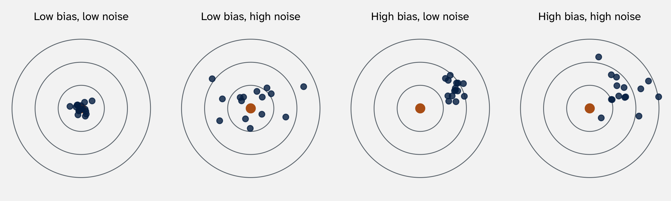
Week 1: our dataset is one run of the process. Imagine 15 runs of the résumé study, with new employers each time. Each blue dot is one run’s estimate

The orange dot is the estimand, the true effect. Each blue dot is the estimate from one run of the study. Simulated data
\[ \underbrace{3.2 \text{ points}}_{\text{estimate}} = \underbrace{\text{true effect}}_{\text{estimand}} + \underbrace{0}_{\text{bias}} + \underbrace{\text{noise}}_{\text{luck of the draw}} \]
Randomization makes the bias zero, on average. The two piles of résumés are alike on average, so the comparison isn’t tilted
Noise is luck, and luck cancels out. With 10 employers, one odd employer moves the average a lot. With 5,000, it barely moves it. Last week’s standard error measures it
Bias doesn’t cancel. If the comparison itself is off, every new data point repeats the same mistake.
Today: two big sources of bias, confounding and measurement
| Country | Year | Polity score | Democracy? | GDP per capita ($1,000s) | New civil war |
|---|---|---|---|---|---|
| India | 1989 | 8 | Yes | 1.2 | 1 |
| Peru | 1981 | 7 | Yes | 3.1 | 1 |
| Rwanda | 1990 | -7 | No | 0.8 | 1 |
| China | 1998 | -7 | No | 2.5 | 0 |
| Switzerland | 1998 | 10 | Yes | 16.1 | 0 |
| United States | 1998 | 10 | Yes | 20.6 | 0 |
The unit of analysis is the country-year. civil_war is 1 in a year a civil war began
Polity score: experts rate how democratic a country’s institutions are, from –10 (full autocracy) to 10 (full democracy). We call a score above 5 a democracy

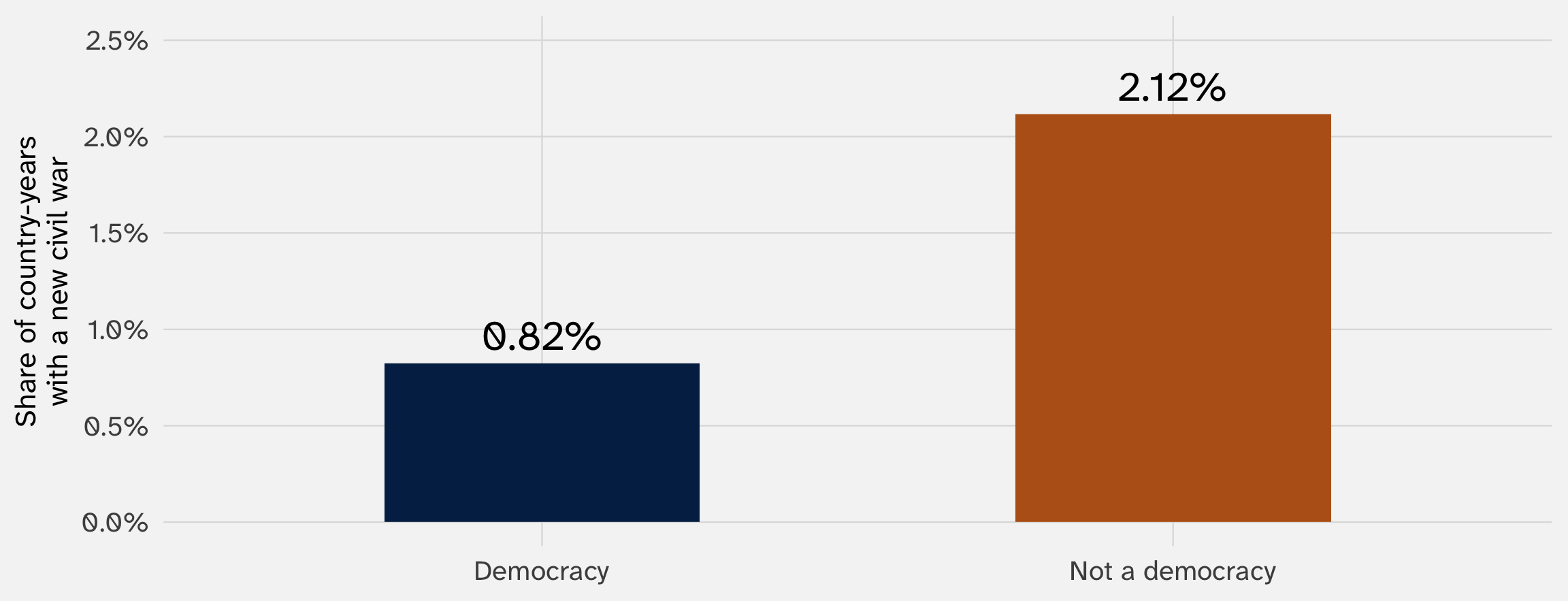
Country-years, 1945–1999. A country-year counts as a democracy if its Polity score is above 5 (on a scale from –10 to 10). Data: Fearon and Laitin (2003), via the juanr package
| In this question | |
|---|---|
| Estimand | How much being a democracy changes a country’s chance of a civil war starting |
| Estimator | Difference in means: the war rate in democracies minus the rate in non-democracies |
| Estimate | -1.3 points |
What might bias this estimate?
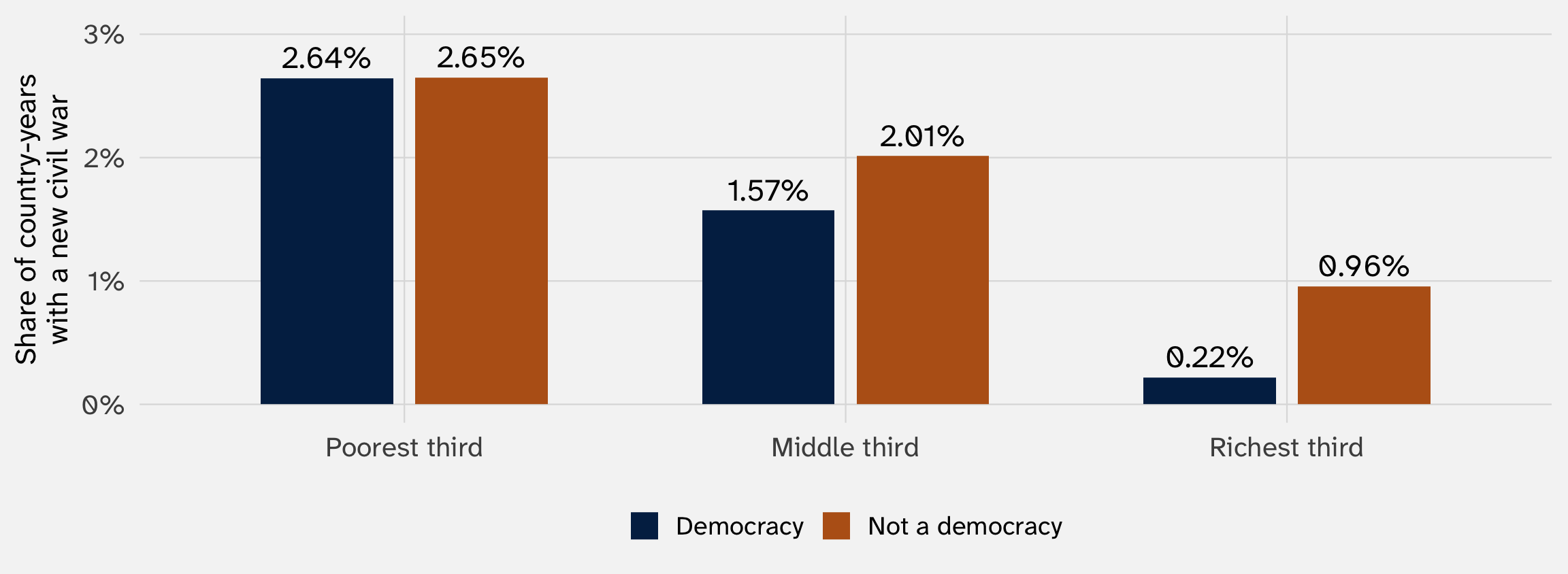
Average GDP per capita: $6.2k in democracies vs. $2.4k in non-democracies
A new civil war began in 2.6% of the poorest third of country-years, and 0.5% of the richest third
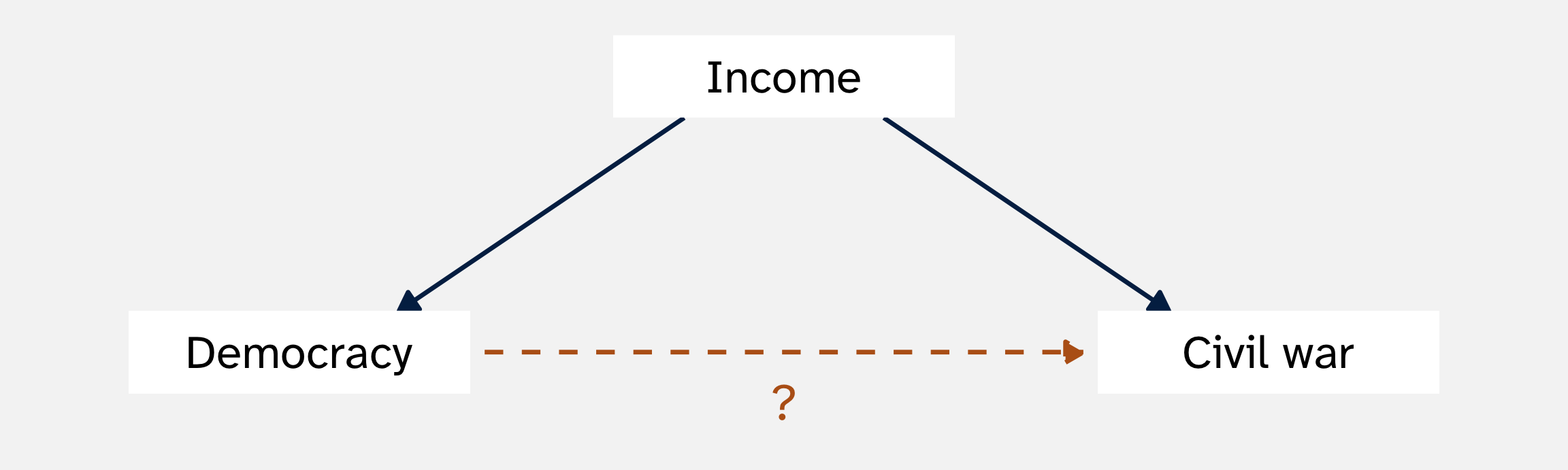
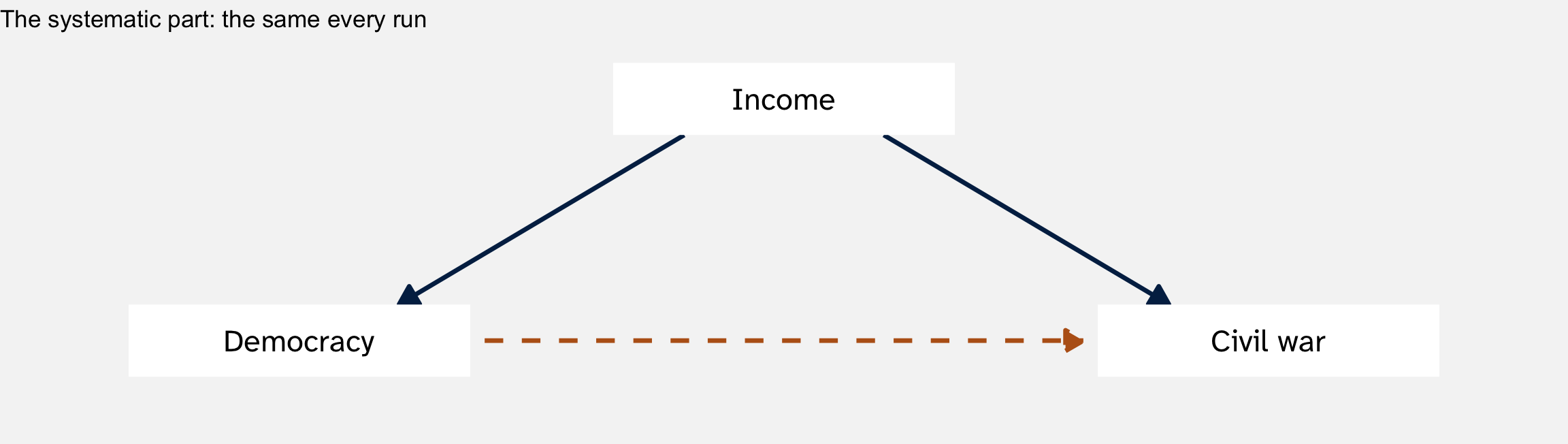
The gap between democracies and non-democracies could be income, not democracy

A confounder is a variable that affects both the treatment (\(X\)) and the outcome (\(Y\))
Confounding is systematic part of DGP: the data is being generated such that democracies tend to be wealthier and have more/less conflict
More data won’t fix it: 6 million country-years would still mix democracy with income
\[ \underbrace{\text{Difference in means}}_{\text{estimate}} = \underbrace{\text{Effect of democracy on democracies}}_{\text{estimand}} + \underbrace{\text{Baseline difference}}_{\text{bias}} + \text{Noise} \]
Baseline difference: how much less civil war the democracies would have had even without democracy, compared to the non-democracies (Bueno de Mesquita and Fowler 2021, 166)
Democracies are richer, so they’d have fewer civil wars anyway. The baseline difference is negative, and it makes democracy look more peaceful than it is
Imagine if we could see the counterfactual:
| Civil war rate | |
|---|---|
| Democracies, as democracies | 1.0% |
| Democracies, if they had not been democracies | 1.5% (we never see this) |
| Non-democracies, as non-democracies | 2.5% |
\[ \underbrace{1.0 - 2.5}_{\text{what we see: } -1.5} = \underbrace{(1.0 - 1.5)}_{\text{effect on democracies: } -0.5} + \underbrace{(1.5 - 2.5)}_{\text{baseline difference: } -1.0} \]
Two-thirds of the gap we see turns out to be bias
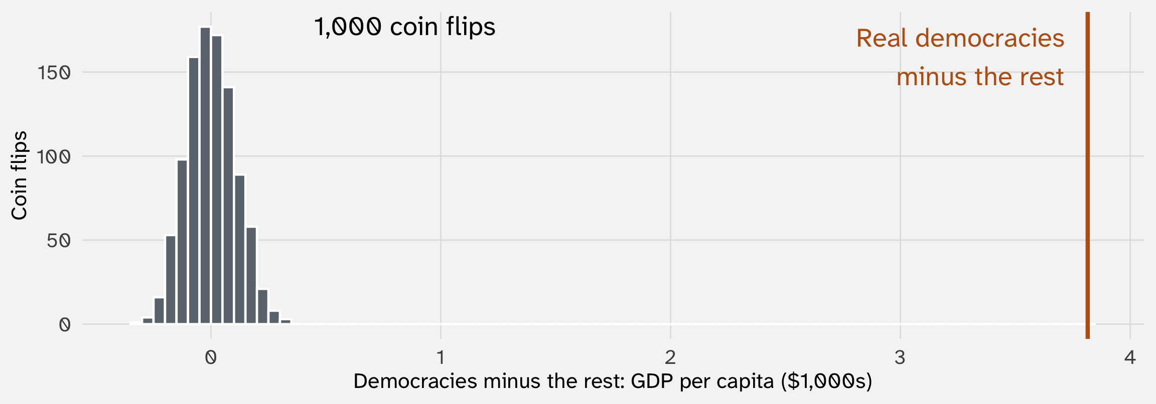
If a coin flip had picked the democracies, they’d be no richer than the rest, on average. Let’s simulate this:
# A tibble: 6,343 × 5
country year civil_war democracy coin
<chr> <dbl> <dbl> <chr> <chr>
1 USA 1945 0 Democracy Not a democracy
2 USA 1946 0 Democracy Democracy
3 USA 1947 0 Democracy Democracy
4 USA 1948 0 Democracy Democracy
5 USA 1949 0 Democracy Not a democracy
# ℹ 6,338 more rows
Sampling
sample() picks among the elements in x, n times, each time returning its pick to the x (“replace = TRUE”)
# A tibble: 2 × 2
democracy gdp
<chr> <dbl>
1 Democracy 6.19
2 Not a democracy 2.37
Real democracies vs. the rest: $6.2k vs. $2.4k.

Real GDP per capita for 6,343 country-years; the democracy labels come from simulated coin flips. Data: Fearon and Laitin (2003), via the juanr package
Every coin-flip gap falls within $0.32k of zero. Randomization turns a systematic difference (income) into a random one (the luck of the flip), and random differences average out
Two questions about a confounder:


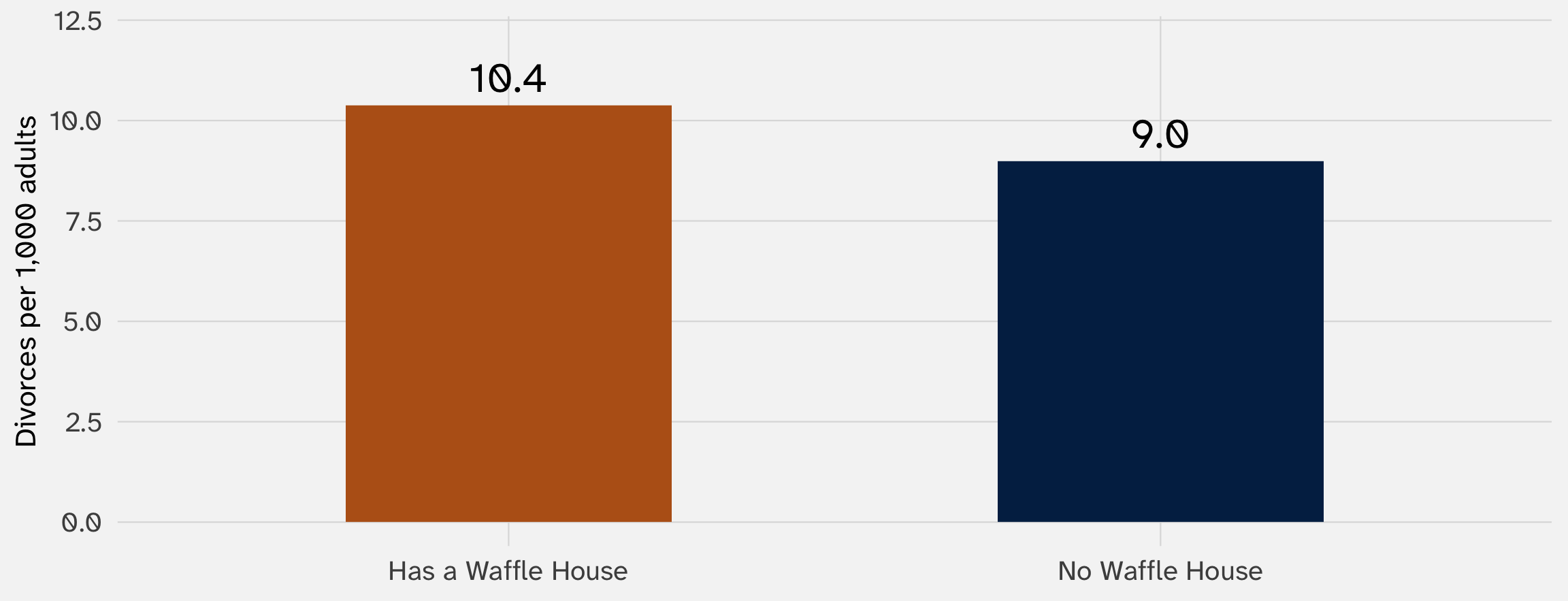
Average divorce rate in the 25 states with at least one Waffle House and the 25 without. Data: McElreath (2020)
Do cheap, delicious waffles put marriages at risk?
| Region | Has a Waffle House | No Waffle House |
|---|---|---|
| Not South | 11 | 25 |
| South | 14 | 0 |
The South has more divorce and more Waffle Houses. It’s a confounder
And no Southern state lacks a Waffle House, so we can’t even compare within the South. No variation, no comparison
Ask the two questions about the South:
So the Waffle House states would have more divorce even with no waffles. They start ahead, so the baseline difference is positive
The gap we see is the effect of waffles plus that head start
Positive bias: waffles look worse for marriage than they are
In a simulation, we make up the data-generating process ourselves, so we know the truth
set.seed(1181) # makes the random draws the same every time we run this
fake_states = tibble(
south = sample(c(0, 1), size = 50, replace = TRUE, prob = c(0.7, 0.3)),
waffle = rnorm(50, mean = 20, sd = 4), # Waffle Houses per million residents
divorce = rnorm(50, mean = 9, sd = 1.5) # divorces per 1,000 adults
)
In plain words
sample() makes about 3 in 10 states Southern
rnorm() gives each state a waffle rate and a divorce rate: a center plus its own random nudge
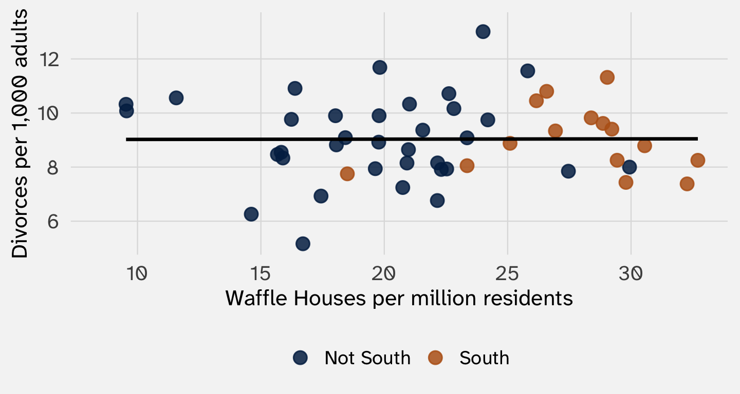
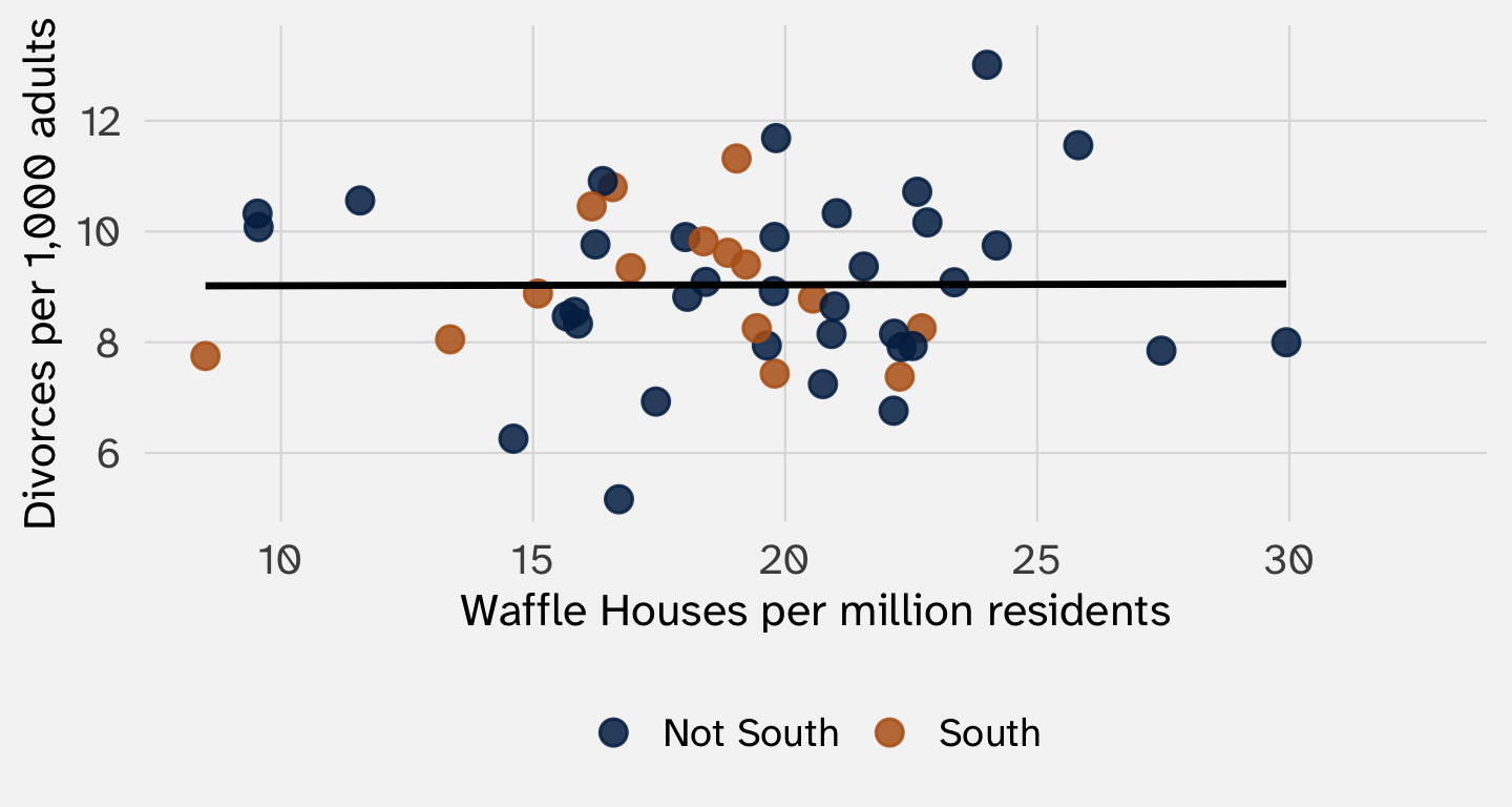
No confounding; the line is flat

The waffle line
Systematic part: 20, plus 10 in the South. That + 10 * south is the arrow from the South to waffles
Random part: each state’s nudge (sd = 4)
The Southern states slide right. Divorce still has nothing to do with anything

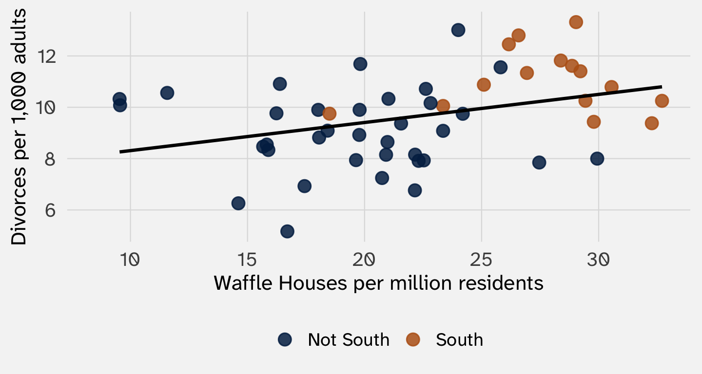
The divorce line
Systematic part: 9, plus 2 in the South
Random part: each state’s nudge (sd = 1.5)
waffle appears in neither
The Southern states move up. Now the states with the most waffles have the most divorce

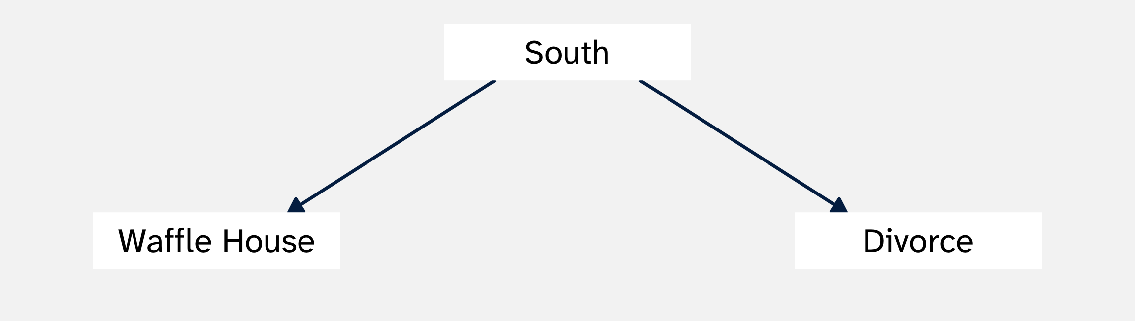
The arrows are the systematic part. waffle line: an arrow from the South to waffles. divorce line: an arrow from the South to divorce
waffle appears in no systematic part, so no arrow runs from waffles to divorce. The true effect is zero. We know the estimand
The slope of the line from step 3: a state with 10 more Waffle Houses per million residents has about 1.1 more divorces per 1,000 adults
\[ \underbrace{0.11}_{\text{estimate}} = \underbrace{0}_{\text{estimand}} + \text{bias} + \text{noise} \]
The South raises waffles (+) and raises divorce (+). We guessed positive bias, and that’s what we got

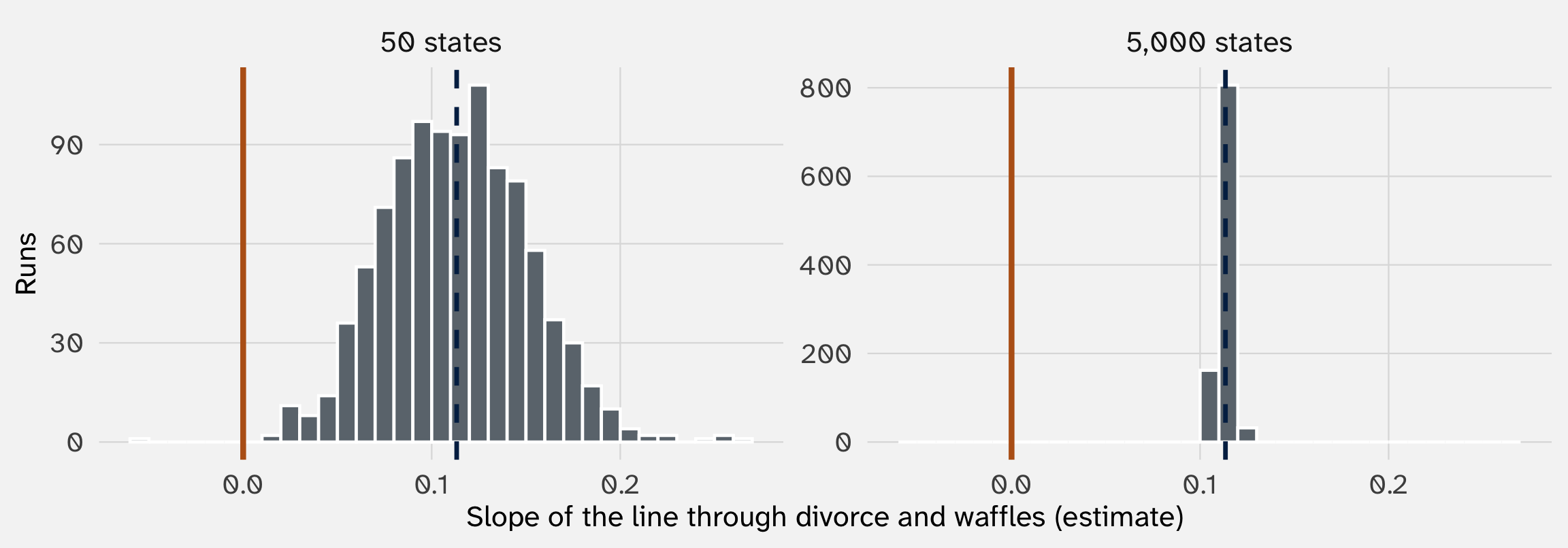
Orange line: the true effect (zero). Dashed line: the average estimate. Simulated data
Each rerun keeps the systematic part and redraws the random part. The confounding is in the systematic part, so the bias comes back every run: the slopes center on about 0.11, not zero. More states only tighten the spread
fake_states |>
mutate(region = if_else(south == 1, "South", "Not South")) |>
ggplot(aes(x = waffle, y = divorce, color = region)) + # color splits the data by region
geom_point() +
geom_smooth(method = "lm", se = FALSE) + # so we get one line per region
labs(x = "Waffle Houses per million residents", y = "Divorces per 1,000", color = NULL)
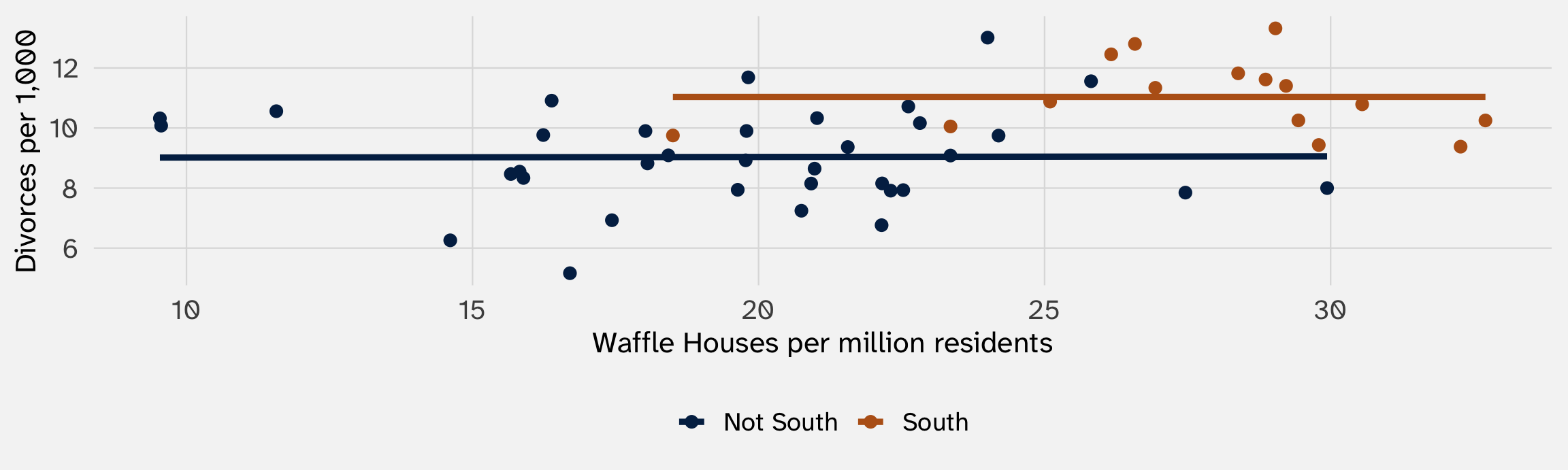
Within each region, the line is flat. The slope of 0.11 through all the states was the South, not waffles. Holding the South fixed removes the bias
set.seed(1181)
fake_states = tibble(
south = sample(c(0, 1), size = 50, replace = TRUE, prob = c(0.7, 0.3)),
waffle = rnorm(50, mean = 20, sd = 4) + 10 * south,
divorce = rnorm(50, mean = 9, sd = 1.5) + 2 * south
)
ggplot(fake_states, aes(x = waffle, y = divorce)) +
geom_point(aes(color = factor(south))) +
geom_smooth(method = "lm", se = FALSE)color = factor(south) into ggplot(aes()). Does the tilt go away?+ 0.1 * waffle to the end of the divorce line. Is the line through all the states steeper than the lines within each region?Ask two questions about a confounder: does it push the treatment up or down? Does it push the outcome up or down?
| Confounder raises the outcome | Confounder lowers the outcome | |
|---|---|---|
| Confounder raises the chance of treatment | Positive bias: estimate too high | Negative bias: estimate too low |
| Confounder lowers the chance of treatment | Negative bias: estimate too low | Positive bias: estimate too high |
Same direction: positive bias. Opposite directions: negative bias (Bueno de Mesquita and Fowler 2021, 177–78)
| What income does | Sign | |
|---|---|---|
| Effect on the treatment (democracy) | Richer countries are more often democracies | + |
| Effect on the outcome (civil war) | Richer countries have fewer civil wars | – |
| Bias | – |
Democracies are mostly rich, and rich countries have fewer civil wars anyway. The democracies start ahead on peace, so the baseline difference is negative
Negative bias: our estimate (-1.3 points) is lower than the true effect. The true effect is closer to zero, or even above it
Prediction: hold income fixed, and the gap should shrink. Let’s check
library(juanr)
wars = fearon |>
filter(!is.na(polity2), !is.na(gdp_cap)) |> # drop rows missing either one
mutate(democracy = if_else(polity2 > 5, "Democracy", "Not a democracy"),
civil_war = if_else(onset > 0, 1, 0),
income = ntile(gdp_cap, 3)) # 3 equal-sized groups: 1 = poorest
wars |>
group_by(democracy) |>
summarize(war_rate = mean(civil_war))summarize()income to group_by(). Does the gap survive within each income group?
Income groups are thirds of all country-years by GDP per capita, 1945–1999. Data: Fearon and Laitin (2003), via the juanr package
All countries: a gap of -1.29 points. Within each income group: -0.01, -0.44, and -0.74
Week 1: adding a control for respondent sex barely moved the résumé estimate, even though sex could affect \(Pr(callBack)\)
Why? because the names were randomized
Here, holding income (roughly) fixed moves the estimate a lot, in the direction we predicted. That’s the sign of a confounder
POL 212 does this with regression. The logic is the same: compare democracies and non-democracies that are alike on income
Name a likely confounder, sign the bias, and say what it does to the estimate
| Comparison | Likely culprit | Effect on the treatment | Effect on the outcome | Bias |
|---|---|---|---|---|
| Phone calls and turnout | Voted in past elections | + campaigns call regular voters | + | Up: calls look more effective than they are |
| Peacekeepers and violence | How bad the war was | + peacekeepers go to the hardest cases | + | Up: peacekeepers look harmful |
| Tutoring and test scores | Struggling in school | + struggling students get tutored | – | Down: tutoring looks harmful |
| Democracy and civil war | Civil war itself (reverse causality) | – war erodes democracy | + | Down: democracy looks more peaceful |
Income pushes the bias down. Population pushes it up: democracies are a bit bigger, and bigger countries have more civil wars
Which push wins? Hard to guess. For confounders no one measured, impossible to check
“Negative” says the estimate is too low, not by how much
A big bias can even flip the sign. Police go where crime is high, so places with more police can have more crime, even if police reduce it (Bueno de Mesquita and Fowler 2021, 176–77)
Signing the bias is useful, but not a fix. Take POL 285 to learn more about how to address these issues
Start from the waffle code:
Week 1’s definition had two halves:
“A data-generating process (DGP) is a rule or set of rules governing the social or political events that an analyst wishes to study and the rules by which observations of its results come to be represented in a dataset.”
— Gailmard (2014, 70)
So far today: the first half, the events themselves. Now the second half: how a civil war, a regime, or a person’s race turns into a number in our data
That step has its own systematic part and its own random part
| Concept | What we measured |
|---|---|
| Race (week 1) | The name on a résumé |
| Democracy | A Polity score above 5 |
| Wealth | GDP per capita |
| Civil war | Fighting between a state and rebels that killed at least 1,000 people |
Before we compare anything, ask: does the number capture the concept?
| Type | What the numbers mean | Example |
|---|---|---|
| Nominal | Just labels | Country, region |
| Ordinal | Order, but the gaps may not be equal | Polity score, “agree/disagree” survey scales |
| Interval | Equal gaps, but no true zero | Year |
| Ratio | Equal gaps and a true zero | GDP per capita, population |
These four types come from Stevens (1946)
Measuring democracy as ordinal or interval has consequences
| Democracy if Polity is above… | Share counted as democracies | War rate, democracies | War rate, the rest | Gap (points) |
|---|---|---|---|---|
| 0 | 43% | 1.29% | 1.96% | -0.67 |
| 5 | 34% | 0.82% | 2.12% | -1.29 |
| 9 | 19% | 0.33% | 1.98% | -1.65 |
A cutoff turns a scale into a yes/no. It’s a choice, and here it moves the gap by more than a point
For the fuller version, see Adcock and Collier (2001)
| Country | Polity score | Democracy? (above 5) |
|---|---|---|
| United States | 10 | Yes |
| United Kingdom | 10 | Yes |
| South Africa | 9 | Yes |
| India | 9 | Yes |
| Brazil | 8 | Yes |
| Mexico | 6 | Yes |
| Russia | 4 | No |
| Iran | 3 | No |
| Indonesia | -5 | No |
| China | -7 | No |
The United States and the UK at the top, China at the bottom. It passes the sniff test, a low bar
| Country | Years | Polity score | Who couldn’t vote |
|---|---|---|---|
| Switzerland | 1950–1970 | 10 | Women, in federal elections, until 1971 |
| United States | 1945–1964 | 10 | Most Black Southerners, until the Voting Rights Act of 1965 |
Polity scores competition and limits on the executive, not how many people can vote. It misses part of what most of us mean by democracy (Paxton 2000)
Does this matter? It depends on your theory; what aspects of democracy does your theory depend on? How exactly does democracy affect your outcome?
Week 1: the name on a résumé measured race. But a name also signals class (Fryer and Levitt 2004)
A measure that picks up a second concept fails this test: we can’t tell which concept moved the outcome
A second check: does the measure relate to other things the way the concept should? A good democracy measure should agree with other democracy measures, like V-Dem from week 1
\[ \text{Measured value} = \text{True value} + \text{Bias} + \text{Noise} \]
Misses in the same direction every time
We are interested in broad participation, but Polity gives Switzerland a 10 before women could vote
Misses at random
Two coders read the same country differently; a survey respondent answers differently on another day

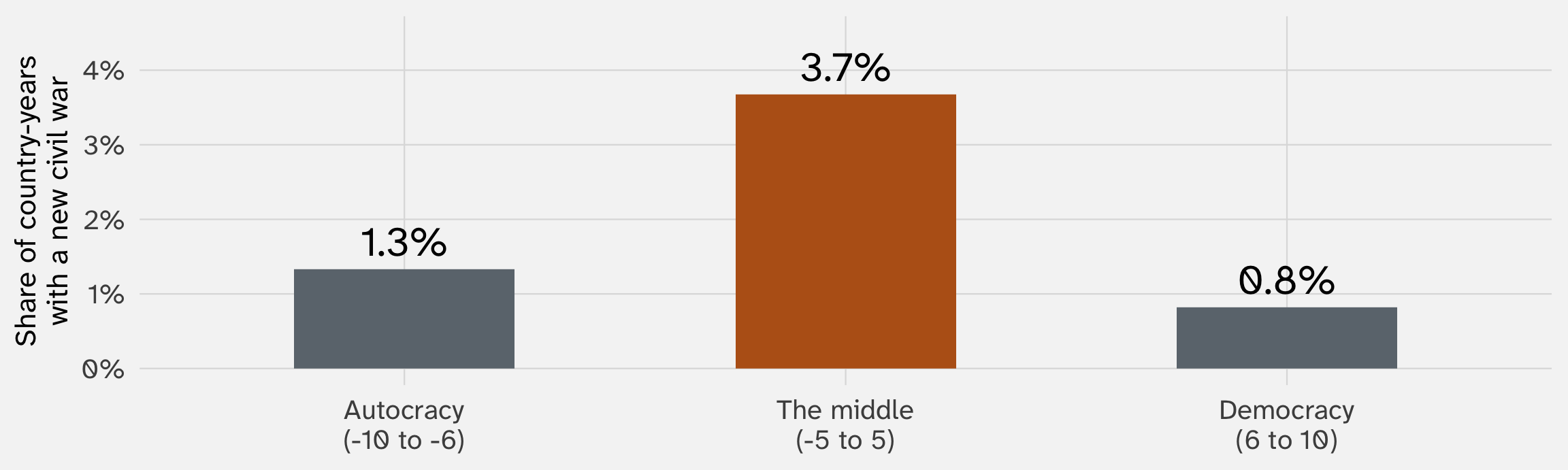
Country-years, 1945–1999, by Polity score. Data: Fearon and Laitin (2003), via the juanr package
A well-known finding: regimes in the middle (“anocracies”) have the most violence (Hegre et al. 2001). The story: dictators can crush resistance, and democracies give people a peaceful way to seek reform. Regimes in the middle can do neither
Two of Polity’s parts have a “factional” category, for politics that is “intense, hostile, and frequently violent” (Polity’s codebook, quoted in Vreeland 2008)

So a country sliding into violence gets scored toward the middle. The treatment is measured partly with the outcome: the bias in the measure depends on the violence
Drop those parts, and the link between the middle and civil war disappears (Vreeland 2008)
Is there more violence in the middle?
A more recent study, using machine learning, finds the pattern is still there (Jones and Lupu 2018)
Much conflict data comes from news reports. Violence far from reporters is more likely to be missed (Weidmann 2016)
Areas with cell phone coverage seem to have more violence (Pierskalla and Hollenbach 2013). Part of that “effect” is that violence in covered areas gets reported more (Weidmann 2016)
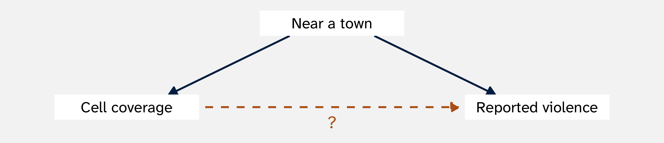
A biased measure of the outcome can create an effect that isn’t there
Noise in the outcome and noise in the treatment can produce different patterns:
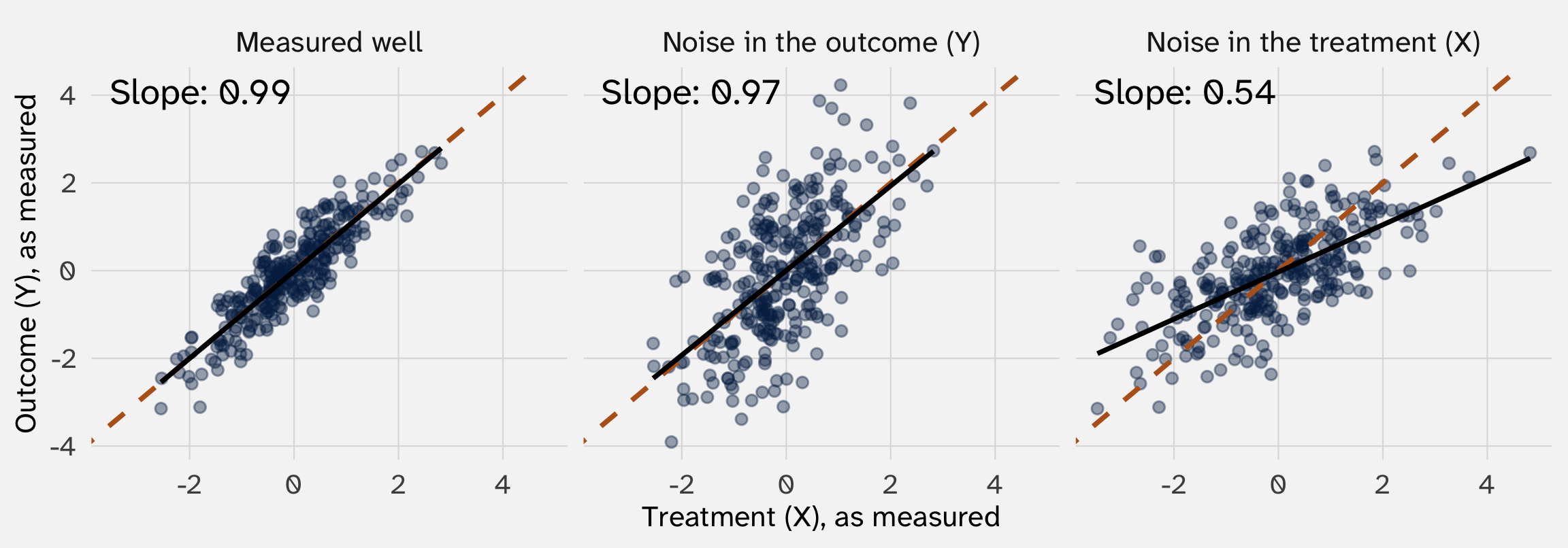
Orange dashed line: the true effect (a slope of 1). Black line: the line through what we measured. Simulated data
Noise in \(Y\) leaves the slope near 1. Noise in \(X\) cuts it about in half
Pushes each point up or down at random
At any value of X, the ups and downs cancel. The line stays put; we just see it less clearly. More noise, no bias
Pushes each point left or right at random
The points at the far right are partly there because of a big random push. Their Y is ordinary, so the right end of the line sags. The line flattens toward zero: bias
POL 211 · Fall 2026