| Name on résumé | Sex | Race of name | call |
|---|---|---|---|
| Allison | Female | White-sounding | 0 |
| Kristen | Female | White-sounding | 0 |
| Lakisha | Female | African American-sounding | 0 |
| Latonya | Female | African American-sounding | 0 |
| Carrie | Female | White-sounding | 0 |
| Jay | Male | White-sounding | 0 |
Introduction
POL 211 · Week 1
Juan F. Tellez
University of California, Davis
September 29, 2026
Today
- A working example
- A common terminology, causality
- How the world makes data (DGPs)
Plus: how the course works, and a 10-minute break
A working example
Bertrand and Mullainathan (2004) sent about 5,000 fake résumés to real job ads
Half got white-sounding names
Emily, Greg, Anne
Half got African American-sounding names
Lakisha, Jamal, Tamika
The names were assigned at random. Then they waited to see which résumés got a callback
Each row is one résumé sent to one employer
4,870 résumés in all. In the data, call is 1 for a callback and 0 otherwise. Of all résumés, 8% got a call back
What was the callback rate for each group?
We can take the conditional mean of each group:
# A tibble: 2 × 3
  race  callback_rate     n
  <chr>         <dbl> <int>
1 black        0.0645  2435
2 white        0.0965  2435
Remember…
The average of a 0/1 variable is a proportion: the share of résumés that got a call
White-sounding names got 50% more callbacks
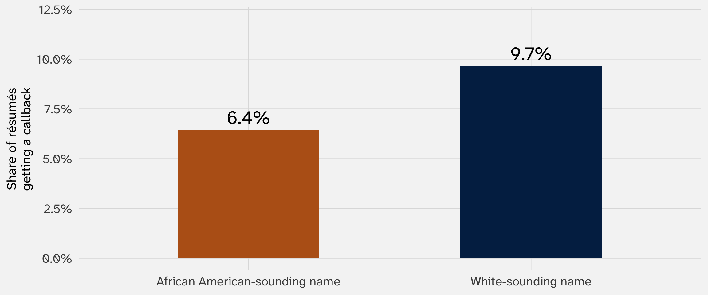
What is the effect of having the “wrong” kind of name?
\[ \underbrace{9.7\%}_{\text{white-sounding}} \; - \; \underbrace{6.4\%}_{\text{African American-sounding}} \; = \; 3.2 \text{ points} \]
This difference in means is our estimate of the effect of race on callbacks
A regression gives us the same number
\[ \text{Callback}_i = \alpha + \beta \cdot \text{African American name}_i + \varepsilon_i \]
\(\alpha\) is the callback rate for white-sounding names. \(\beta\) is how much it changes when the name changes
The slope tells us how much Y changes when X changes
| Callback (1) | Callback (2) | |
|---|---|---|
| African American-sounding name | -0.032 | -0.032 |
| (0.008) | (0.008) | |
| Female applicant | 0.009 | |
| (0.009) | ||
| Intercept | 0.097 | 0.090 |
| (0.006) | (0.009) | |
| Résumés | 4,870 | 4,870 |
Linear regression. Outcome: callback = 1 if the employer called back, 0 if not. Standard errors in parentheses.
An African American-sounding name lowers the callback rate by 3.2 points
Accounting for other variables barely moves the estimate
| Callback (1) | Callback (2) | |
|---|---|---|
| African American-sounding name | -0.032 | -0.032 |
| (0.008) | (0.008) | |
| Female applicant | 0.009 | |
| (0.009) | ||
| Intercept | 0.097 | 0.090 |
| (0.006) | (0.009) | |
| Résumés | 4,870 | 4,870 |
Linear regression. Outcome: callback = 1 if the employer called back, 0 if not. Standard errors in parentheses.
Column 2 adds the applicant’s sex. Our effect estimate is now net of differences in male and female applicants’ likelihood of being chosen. The estimate hardly changes, because the names were randomized
The standard error says how far a new sample could move the estimate
| Callback (1) | Callback (2) | |
|---|---|---|
| African American-sounding name | -0.032 | -0.032 |
| (0.008) | (0.008) | |
| Female applicant | 0.009 | |
| (0.009) | ||
| Intercept | 0.097 | 0.090 |
| (0.006) | (0.009) | |
| Résumés | 4,870 | 4,870 |
Linear regression. Outcome: callback = 1 if the employer called back, 0 if not. Standard errors in parentheses.
If we ran the study again with different employers, we’d get a slightly different number. The standard error says how different: a 95% confidence interval from -4.7 to -1.7 points
We can read it as causal because the names were randomized
Randomization
The two groups of résumés were alike, on average, in every way except the name
So
A difference in callbacks can’t come from experience, schooling, or the jobs they applied to
Most of the data you’ll work with isn’t an experiment. Then this question gets much harder
What else could a name signal?
Randomization worked: the résumés differ only in the name. This shows that employers discriminate against applicants when they can tell that they are African-American
What objection(s) could a skeptic raise here?
A skeptic would say the name signals class, not only race
What a name can signal
Race, but also the parents’ income and education, and where someone grew up
Distinctively African American names are more common among children of poorer, less-educated mothers (Fryer and Levitt 2004)
What that does to the estimate
The study may measure a class penalty and a race penalty, mixed together
And when people are asked, not every name in these studies reads as clearly Black (Gaddis 2017)
Two problems
Bundled treatment
Changing the name changes several signals at once (a “bundled treatment”). So we estimate the effect of the whole bundle: race, class, and the rest (Sen and Wasow 2016)
Also a measurement problem
We want to learn about race. The name is how we measure race in this study, and it’s an imperfect measure
The effect is causal. The question is what it’s the effect of
How the course works
How the methods sequence maps onto this study
| Piece of the analysis | Where you learn it |
|---|---|
| Regression to estimate relationships/effects | POL 212 |
| Quantifying uncertainty | POL 212 |
| Controlling for confounds | POL 212, POL285 |
Modeling a 0/1 outcome like call properly |
POL 213 |
| Design-based inference | POL 285 |
POL 211 is the foundation the rest of the sequence stands on
| Course | When | What it adds |
|---|---|---|
| POL 211 | Fall | The foundations: causality, probability, inference |
| POL 212 | Winter | Linear regression (OLS) |
| POL 213 | Spring | Maximum likelihood (MLE): logit, counts, durations |
| POL 285 | Later | Causal inference and research design |
This course is about why and when regression, experiments, inference works
Review website
The required courses are the floor!
My advice, which the rest of the methods faculty would sign on to:
- Front-load methods in your first two years, so you can use them in your dissertation
- Take at least six quarters of methods, and read beyond your courses
If you want methods as a subfield, you must do the extra, harder problems on problem sets and exams. I’d encourage everyone to try them
You learn methods by doing
Learning methods is like learning a language. You have to practice
You will get stuck. That’s normal, and it’s where the learning happens
Come to office hours
Your turn: set up your project for the quarter
- Make a folder for this course, e.g.
pol211/, somewhere other than Downloads - Create an R project in it
- Inside, make four folders:
notes/,data/,figures/,sets/
Write everything for this course inside this project
Your turn: render a file you could turn in
Each problem set, you’ll turn in your .qmd plus one self-contained HTML file
- In your project, make a new Quarto document,
test.qmd, with this header:
- Render it. Find
test.htmlin your project folder: one file, no_filesfolder next to it. That one file is what you turn in to Max - Now delete
test.htmland re-render
Why embed-resources?
embed-resources packs the plots and styling into the one HTML file. Without it, the HTML depends on a local test_files/ folder and will not render correctly on someone else’s machine
What is quantitative social science?
Quantitative methods test positive theories
“In basic and abstract terms, a positive theory in social science asserts that two or more concepts or events are related to each other and specifies the reason why.”
— Gailmard (2014, 4)
Positive theories specify some process, channel, or mechanism through which one concept (\(x\)) causes a change in another (\(y\))
Positive theories can be simple or complex: the effect of \(x\) on \(y\) could depend entirely on \(z\), for instance
Positive questions ask how the world works, not how it should
Positive
Do American employers discriminate on the basis of race?
Does democracy make war less likely?
Normative
Should identity play any role in employment?
Is democracy the best form of government?
Other traditions ask different questions, and qualitative work can be positive too
Different questions
Interpretive work asks what actions and institutions mean to the people involved
Critical theory asks how power shapes the world, and how it could be otherwise
Positive qualitative research
Skocpol’s States and Social Revolutions (1979) compares three revolutions to find the conditions that produce them
That’s a positive theory, tested with cases instead of a dataset
Descriptive studies ask what is; causal studies ask what would change
Descriptive
What is the demographic profile of a Democratic Socialists of America supporter?
How has democracy changed around the world since 1990?
Do counties with more college graduates vote more Democratic?
Causal
Does foreign aid reduce violence?
Would employers discriminate less if the name changed?
Does divided government change how presidents make policy?
The line between descriptive and causal is blurry, scholars fight about it
Many papers describe a pattern and word it carefully: X “is associated with,” “is linked to,” or “predicts” Y
Critics say the question is usually causal anyway. Readers take the pattern as a cause, and the careful wording reduces the burden of proof (Grosz, Rohrer, and Thoemmes 2020; Hernán 2018)
Defenders say good description is a contribution in its own right, and shouldn’t have to pretend to be causal (Gerring 2012)
Is this study descriptive or causal?
“Presidents select from a range of instruments when creating new policies through executive action. We study strategic substitution in this context and argue that presidents use less visible means of unilateral instruments when Congress is likely to scrutinize presidential action. Using data on unilateral orders issued between 1946 and 2020, we report two main findings. First, analyzing presidents’ choice of instruments, we show that presidents are more likely to substitute memoranda and other less visible instruments for executive orders and proclamations during periods of divided government. Second, after accounting for the substitution of executive orders with other instruments, we find that presidents issue greater numbers of directives during divided government than during unified government. These findings provide new evidence about the limitations of the separation of powers as a constraint on presidential unilateralism and highlight the importance of accounting for the variety of instruments through which presidents create unilateral policies.”
— Kaufman and Rogowski (2024, 816)
We ask about the effects of causes, not the causes of effects
What causes Y?
What causes civil war?
What makes people vote?
Does X cause Y?
Does foreign aid reduce violence?
Does a campaign phone call make people vote?
The questions on the left might motivate us, but have too many answers to be useful
The questions on the right force us to be more precise about what we are estimating
Why did World War I happen? Every answer is a “but-for” cause
- The great powers were locked into alliances
- An arms race had built huge armies
- Balkan nationalists wanted the archduke dead
- On the day, his driver took a wrong turn and stopped in front of the assassin
Take away any one, and the war might not have happened. Each is a but-for cause: no X, no Y
Go back far enough and everything “matters”, down to the first fish that crawled out of the sea (Bueno de Mesquita and Fowler 2021)
“Why do wars happen?” has no single answer
Courts face the same problem. A driver who runs a red light is a but-for cause of the crash. So is the fussy baby that made them late. The law adds a judgment call, proximate cause, to blame the driver and not the child
So instead of “why do wars happen?” we focus on a proximate cause: do alliances make war more likely?
We study the effects of causes, not the causes of effects
Let’s take a 10-minute break
What do we mean by a cause?
Many of the questions we care about are causal
International relations: do peacekeepers reduce conflict in countries emerging from civil war, or are they ineffective?
Comparative politics: do elections reduce or increase corruption?
American politics: do voter ID laws hurt turnout?
Our study: does the name on a résumé change an applicant’s employment opportunities?
A definition of causality
In this class, we say X causes Y if…
An intervention that changes the value of X produces a probabilistic change in Y
- Intervention: X is being changed or altered
- Probabilistic: Y should change on average, but need not in every instance
“A causal effect is a change in some feature of the world that would result from a change to some other feature of the world.”
— Bueno de Mesquita and Fowler (2021, 37)
The effect of aspirin
Aspirin causes a reduction in fever symptoms
Intervention: someone takes aspirin. We give it to them, sneak it into their food, etc.
Probabilistic: aspirin doesn’t work every time. But in general, on average, taking aspirin \(\rightarrow\) less fever
What about this one?
Democratic institutions reduce the incidence of interstate war
Or this one?
Race significantly shapes people’s political preferences
We call X the treatment and Y the outcome
| We call it | What it is | Examples | |
|---|---|---|---|
| \(X\) | Treatment | The thing that might change an outcome | The name on a résumé, minimum wage laws, voter ID laws, peacekeepers |
| \(Y\) | Outcome | The thing a treatment might affect | Callbacks, employment, turnout, violence |
You’ll also see other names for these in papers and other courses:
- \(X\): the independent variable, exposure, or predictor
- \(Y\): the dependent variable or response
We’ll say treatment and outcome, even when no one assigned the treatment
Treatment makes clear that we are drawing a comparison between treated and control units
This works when X comes in amounts, too. “Treated” means more of it and “control” means less: a state with a $15 minimum wage vs. a state with $10
A causal effect compares two worlds
The world where the treatment happens
The résumé goes out with the name Lakisha
The world where it doesn’t
The same résumé, to the same employer, with the name Emily
Our test is always a comparison between a world where the treatment happens and a world where it doesn’t
The effect of the name is the difference between these two worlds
One of the two worlds is always counterfactual: we can only estimate what would have happened
Causal terminology
| Symbol | Read it as | In the résumé study |
|---|---|---|
| \(i\) | “unit \(i\)” | one résumé: \(i = 1, 2, \ldots,\) 4,870 |
| \(X_i\) | “the treatment for unit \(i\)” | AA if it has an African American-sounding name, W if white-sounding |
| \(Y_i\) | “the outcome for unit \(i\)” | 1 if the employer called back, 0 if not |
The subscript \(i\) just says which résumé we’re talking about. \(Y_7\) is whether résumé #7 got a callback
What’s in the parentheses says which treatment. \(Y_2(\text{AA})\) is whether résumé #2 would get a callback if it had an African American-sounding name
This is purely theoretical: what could happen under each treatment
Potential outcomes: what would happen under each treatment
\(Y_i(\text{AA})\)
Read: “Y of i, with an African American-sounding name”
The callback résumé \(i\) would get if it had an African American-sounding name (\(X_i = \text{AA}\))
\(Y_i(\text{W})\)
Read: “Y of i, with a white-sounding name”
The callback résumé \(i\) would get if it had a white-sounding name (\(X_i = \text{W}\))
Every résumé has both, whichever name it actually got
They’re called potential outcomes because only one of them will happen (Holland 1986)
For résumé #1, the name costs a callback
Suppose résumé #1 would get a callback with the name Emily, but not with the name Lakisha:
\[ Y_1(\text{W}) = 1 \qquad Y_1(\text{AA}) = 0 \]
The effect of the name on résumé #1 is the difference:
\[ \tau_1 = Y_1(\text{AA}) - Y_1(\text{W}) = 0 - 1 = -1 \]
\(\tau\) (“tau”) is the individual causal effect. Here, the African American-sounding name took away the callback
Every résumé has its own effect
If we could see both worlds for five résumés (made-up numbers):
| Résumé | \(Y_i(\text{W})\): white name | \(Y_i(\text{AA})\): African American name | Effect \(\tau_i = Y_i(\text{AA}) - Y_i(\text{W})\) |
|---|---|---|---|
| 1 | 1 | 0 | \(-1\) |
| 2 | 0 | 0 | 0 |
| 3 | 1 | 1 | 0 |
| 4 | 0 | 0 | 0 |
| 5 | 1 | 0 | \(-1\) |
For résumés 2, 3, and 4, the name changes nothing. For 1 and 5, it costs a callback
We never see both worlds: the fundamental problem of causal inference
Each résumé goes out with only one name:
| Résumé | \(Y_i(\text{W})\): white name | \(Y_i(\text{AA})\): African American name | Effect \(\tau_i\) |
|---|---|---|---|
| 1 | ? | 0 | ? |
| 2 | 0 | ? | ? |
| 3 | ? | 1 | ? |
| 4 | 0 | ? | ? |
| 5 | 1 | ? | ? |
We see \(Y_i(\text{AA})\) if the résumé got an African American-sounding name, and \(Y_i(\text{W})\) if it got a white-sounding one. Never both. So we can never see a single \(\tau_i\) (Bueno de Mesquita and Fowler 2021, 41)
This is known as the fundamental problem of causal inference (Holland 1986, 947)
We can’t learn any one résumé’s effect, but we can learn the average
One résumé’s effect, \(\tau_i\), needs both of its outcomes. One is always missing, and no amount of data fills in that cell
The average effect doesn’t need pairs. The average of the differences equals the difference of the averages:
\[ \underbrace{\text{average of } \tau_i}_{\text{average effect}} \; = \; \text{average of } Y_i(\text{AA}) \; - \; \text{average of } Y_i(\text{W}) \]
| Bike | Bus | Bus \(-\) bike | |
|---|---|---|---|
| You | 10 | 20 | 10 |
| Your roommate | 15 | 15 | 0 |
| Your friend | 20 | 40 | 20 |
| Average | 15 | 25 | 10 |
Average of the differences: \((10 + 0 + 20) / 3 = 10\)
Difference of the averages: \(25 - 15 = 10\)
So we don’t need 4,870 matched pairs. We need two averages, and an average is something we can estimate from a group
Randomization lets each group stand in for the missing world
We never see all résumés with an African American-sounding name. So we borrow a group:
| Group | What we see | What we use it to stand in for |
|---|---|---|
| Got an AA name | Their callbacks with an AA name | What all résumés would get with an AA name |
| Got a W name | Their callbacks with a W name | What all résumés would get with a W name |
This is an assumption: the two groups are alike, on average, in everything but the name. Randomization makes it true. A coin flip can’t pick the better résumés or the friendlier employers
So the 3.2-point gap estimates the average effect. Without random assignment, the groups can differ in other ways, and the borrowed averages mislead us
A cause doesn’t have to change every outcome
One common skeptical reaction to evidence of an average effect is to point to counterexamples (“I did (did not) get vaxxed and still (did not) get the flu”)
Imagine 100 résumés, sorted by how their employer would respond (potential outcomes):
| Type of résumé | \(Y_i(\text{W})\): white name | \(Y_i(\text{AA})\): African American name | Effect | How many |
|---|---|---|---|---|
| Called either way | 1 | 1 | 0 | 6 |
| Never called | 0 | 0 | 0 | 91 |
| Called only as Emily | 1 | 0 | \(-1\) | 3 |
The average effect is \(-3/100\): 3 points. Yet for 97 of the 100 résumés, the name changes nothing
So “I know a Lakisha who got a callback” doesn’t show that names don’t matter. A counterexample only sinks a claim that X always changes Y (Sekhon 2004)
To make a comparison, we need variation
What is wrong with the following conclusion?
“In Bertrand and Mullainathan (2004), 90% of applicants with white-sounding names don’t get a callback. So a white-sounding name doesn’t help”
| Name on the résumé | No callback |
|---|---|
| White-sounding | 90.3% |
| African American-sounding | 93.6% |
The fact is true. But it isn’t evidence that the name doesn’t matter. You need the résumés with the other name
Without variation in treatment (\(X\)), there’s no comparison
Without variation in Y, there’s no comparison either
The 10,000-hour rule
Gladwell (2008) studied great achievers and found they’d all practiced 10,000 hours
He never looked at people who practiced 10,000 hours and didn’t become great
The Asian tigers
Scholars studied the fastest-growing economies, like South Korea, Taiwan, and Singapore, and found they’d all repressed labor
Add the developing countries that didn’t grow fast, and the link between labor repression and growth disappears (Geddes 1990)
Studying only the cases where the outcome happened is selecting on the dependent variable
The 10,000-hour example is discussed in Bueno de Mesquita and Fowler (2021, 57–64)
What comparison is missing?
Which variation is missing from each claim?
- “Every successful startup founder we interviewed had failed at least once before. Failure breeds success.”
- “Most countries that received UN peacekeepers still had violence five years later. Peacekeeping doesn’t work.”
- “All of the coups in our data happened in countries with weak economies.”
Every causal claim is a comparison. A comparison of what?
Every example today compared two groups: résumés with and without “Lakisha,” countries with and without peacekeepers
The things being compared are the units of analysis
The unit of analysis is the observation, named for what we compare
“Observation” and “unit of analysis” usually point to the same thing: one row
We say unit of analysis because it tells us what we’re comparing
In the résumé study, the units are résumés. They’re the \(i\) in \(Y_i\)
Cross-sectional data: many units at one moment
| Country | Year | Electoral democracy (0–1) | Liberal democracy (0–1) |
|---|---|---|---|
| Brazil | 2023 | 0.78 | 0.69 |
| Colombia | 2023 | 0.70 | 0.56 |
| Germany | 2023 | 0.86 | 0.81 |
| India | 2023 | 0.38 | 0.28 |
| Japan | 2023 | 0.82 | 0.73 |
| Nigeria | 2023 | 0.49 | 0.33 |
The unit is the country. We compare countries to each other
Time series data: one unit, followed over time
| Country | Year | Electoral democracy (0–1) | Liberal democracy (0–1) |
|---|---|---|---|
| United States of America | 2018 | 0.82 | 0.74 |
| United States of America | 2019 | 0.81 | 0.74 |
| United States of America | 2020 | 0.81 | 0.73 |
| United States of America | 2021 | 0.82 | 0.76 |
| United States of America | 2022 | 0.83 | 0.76 |
| United States of America | 2023 | 0.85 | 0.77 |
The unit is the year. We compare the United States to itself at different times
Panel data: many units, each followed over time
| Country | Year | Electoral democracy (0–1) | Liberal democracy (0–1) |
|---|---|---|---|
| Brazil | 2021 | 0.68 | 0.53 |
| Brazil | 2022 | 0.69 | 0.54 |
| Brazil | 2023 | 0.78 | 0.69 |
| India | 2021 | 0.40 | 0.31 |
| India | 2022 | 0.38 | 0.29 |
| India | 2023 | 0.38 | 0.28 |
The unit is the country-year. We can compare across countries and over time
A panel is a stack of time series, one per country. Or a stack of cross-sections, one per year
The same question can be asked with different units
“Do democracies fight fewer wars?”
- Countries: are democracies at war less often than autocracies?
- Country-years: is a country less likely to go to war in the years it’s a democracy?
- Pairs of countries in a year: are two democracies less likely to fight each other?
Each unit answers a different question. Before you analyze anything, say what a row is. A lot of mistakes start there
How the world makes data
The data we see is what a process left behind
Quantitative social science thinks about data as the result of some process we want to understand
“A data-generating process (DGP) is a rule or set of rules governing the social or political events that an analyst wishes to study and the rules by which observations of its results come to be represented in a dataset.”
— Gailmard (2014, 70)
We never see the process itself. We see its results
This is a metaphysical commitment on the part of social scientists
My two little kids are a data-generating process
What I see
Crying, complaining, laughing, calming down, falling asleep
What I can’t see: the process
Systematic: hunger, tiredness, how long since the last nap, each kid’s personality
Stochastic (random): whatever they decide in the moment. Same kid, same nap, same snack, and one day it’s giggles, the next it’s a meltdown
I learn the process by watching what it produces. Meltdowns bunch up around 5 PM, so hunger is probably part of it. But I’ll never predict every tear
Every DGP has a systematic part and a random part
Systematic
The regular patterns our theories are about
In the résumé study: how much the name changes an employer’s chance of calling back
Stochastic
Everything else
Which manager opened the résumé, their mood that morning, whether the job was already filled
A process with no random part is deterministic. Almost nothing we study works like that
A data-generating activity
| Age | Education | Income ($1,000s) | Owns home | Contacted by a campaign | Voted |
|---|---|---|---|---|---|
| 30 | College degree | 113 | No | No | 0 |
| 76 | College degree | 107 | Yes | Yes | 1 |
| 61 | Some college | 48 | Yes | Yes | 1 |
| 33 | Some college | 72 | No | Yes | 1 |
| 34 | Some college | 102 | No | Yes | 1 |
| 21 | Some college | 86 | Yes | Yes | 0 |
| 57 | College degree | 66 | Yes | No | 1 |
| 28 | High school or less | 27 | No | Yes | 1 |
One row per registered voter; voted is 1 if they voted
1,000 voters in all. Overall turnout: 64%
Your turn: model the process behind who votes
Get voters.csv from week 1 on the course schedule. Save it in data/
- Using
case_when(), write down your best guess of the process: who votes, and who doesn’t? - Check it: what share of people does your model get right?
The best simple models get about 7 in 10 people right
voters |>
  mutate(
    everyone       = 1,
    age_45         = case_when(age >= 45 ~ 1,
                               age < 45 ~ 0),
    age_or_contact = case_when(age >= 45 | contacted == 1 ~ 1,
                               age < 45 & contacted == 0 ~ 0)
  ) |>
  summarize(everyone       = mean(everyone == voted),
            age_45         = mean(age_45 == voted),
            age_or_contact = mean(age_or_contact == voted))
# A tibble: 1 × 3
everyone age_45 age_or_contact
<dbl> <dbl> <dbl>
1 0.642 0.65 0.692Nobody gets close to 100%. Why not?
I made the data in two steps
Step 1, the systematic part: each person gets a chance of voting, \(p_i\), from their traits
\[ \text{score}_i = -2.2 + 0.035 \cdot \text{age}_i + 0.6 \cdot \text{some college}_i + 1.1 \cdot \text{college}_i + 0.5 \cdot \text{homeowner}_i + 0.8 \cdot \text{contacted}_i \]
\[ p_i = \frac{1}{1 + e^{-\text{score}_i}} \qquad \text{(this just squeezes the score between 0 and 1)} \]
Step 2, the random part: each person flips a coin that comes up “vote” with probability \(p_i\)
\[ \text{voted}_i = \begin{cases} 1 & \text{with probability } p_i \\ 0 & \text{with probability } 1 - p_i \end{cases} \]
Two people with the same traits get the same \(p_i\), and can still do different things
Only I can see each person’s chance of voting
| Age | Education | Contacted | Chance of voting | Voted |
|---|---|---|---|---|
| 30 | College degree | No | 49% | 0 |
| 76 | College degree | Yes | 95% | 1 |
| 61 | Some college | Yes | 86% | 1 |
| 33 | Some college | Yes | 59% | 1 |
| 34 | Some college | Yes | 60% | 1 |
| 21 | Some college | Yes | 61% | 0 |
The best anyone could do, even knowing every \(p_i\): predict a vote when the chance is over 50%. That gets 69% right
The random part is why a cause can fail in any one case
In my process, campaign contact raises everyone’s chance of voting. It’s a real cause
Contacted
75% voted
But 25% stayed home anyway
Not contacted
59% voted anyway
Same with the résumés: the name shifts an employer’s chance of calling. Any one employer can still call Lakisha, or skip Emily. That’s the “probabilistic” in our definition of a cause
You can’t tell from the data alone whether the world is random
“It is not possible to determine from a given set of observed data alone whether its DGP is stochastic or deterministic.”
— Gailmard (2014, 72)
We only know the voter process is random because I wrote it
With real data, modeling the world as systematic plus random is a metaphysical commitment we are making (but hopefully one that feels reasonable to you!)
Our dataset is one run of the process
Run the résumé study again, with new employers on new days, and we’d get a different gap. Close to 3.2 points, but not exactly. That’s what the standard error captured
History works the same way:
“If we ‘reran’ the history of France over the relevant time period, the progress of its social revolution would not necessarily be the same as what we have in fact observed. Even France’s history as such is then a realization of a random process.”
— Gailmard (2014, 78)
The rest of the course follows from this
Part 1 (weeks 1–3): what is the systematic part, and what biases our view of it?
Part 2 (weeks 4–6): probability, a language for the random part
Part 3 (weeks 7–9): learning about the process from the data we have
References
Bertrand, Marianne, and Sendhil Mullainathan. 2004. “Are Emily and Greg More Employable Than Lakisha and Jamal? A Field Experiment on Labor Market Discrimination.” American Economic Review 94(4): 991–1013. doi:10.1257/0002828042002561.
Bueno de Mesquita, Ethan, and Anthony Fowler. 2021. Thinking Clearly with Data: A Guide to Quantitative Reasoning and Analysis. Princeton, NJ: Princeton University Press.
Fryer, Roland G., and Steven D. Levitt. 2004. “The Causes and Consequences of Distinctively Black Names.” Quarterly Journal of Economics 119(3): 767–805. doi:10.1162/0033553041502180.
Gaddis, S. Michael. 2017. “How Black Are Lakisha and Jamal? Racial Perceptions from Names Used in Correspondence Audit Studies.” Sociological Science 4: 469–89. doi:10.15195/v4.a19.
Gailmard, Sean. 2014. Statistical Modeling and Inference for Social Science. New York: Cambridge University Press.
Geddes, Barbara. 1990. “How the Cases You Choose Affect the Answers You Get: Selection Bias in Comparative Politics.” Political Analysis 2: 131–50.
Gerring, John. 2012. “Mere Description.” British Journal of Political Science 42(4): 721–46. doi:10.1017/S0007123412000130.
Gladwell, Malcolm. 2008. Outliers: The Story of Success. New York: Little, Brown and Company.
Grosz, Michael P., Julia M. Rohrer, and Felix Thoemmes. 2020. “The Taboo Against Explicit Causal Inference in Nonexperimental Psychology.” Perspectives on Psychological Science 15(5): 1243–55. doi:10.1177/1745691620921521.
Hernán, Miguel A. 2018. “The C-Word: Scientific Euphemisms Do Not Improve Causal Inference from Observational Data.” American Journal of Public Health 108(5): 616–19. doi:10.2105/AJPH.2018.304337.
Holland, Paul W. 1986. “Statistics and Causal Inference.” Journal of the American Statistical Association 81(396): 945–60. doi:10.1080/01621459.1986.10478354.
Imai, Kosuke, and Nora Webb Williams. 2022. Quantitative Social Science: An Introduction in Tidyverse. Princeton, NJ: Princeton University Press.
Kaufman, Aaron R., and Jon C. Rogowski. 2024. “Divided Government, Strategic Substitution, and Presidential Unilateralism.” American Journal of Political Science 68(2): 816–31. doi:10.1111/ajps.12821.
Sekhon, Jasjeet S. 2004. “Quality Meets Quantity: Case Studies, Conditional Probability, and Counterfactuals.” Perspectives on Politics 2(2): 281–93.
Sen, Maya, and Omar Wasow. 2016. “Race as a Bundle of Sticks: Designs That Estimate Effects of Seemingly Immutable Characteristics.” Annual Review of Political Science 19: 499–522. doi:10.1146/annurev-polisci-032015-010015.
Skocpol, Theda. 1979. States and Social Revolutions: A Comparative Analysis of France, Russia, and China. Cambridge: Cambridge University Press.
POL 211 · Fall 2026